basic statistical analysis using R#
Note
This is a non-interactive version of the exercise. If you want to run through the steps yourself and see the outputs, you’ll need to do one of the following:
follow the setup steps and work through the notebook on your own computer
open the workshop materials on binder and work through them online
open an R console or RStudio, copy the lines of code here, and paste them into the console to run them
In this exercise, we’ll take a look at some basic statistical analysis with R - starting with using R to calculate descriptive statistics for our datasets, before moving on to look at a few common examples of hypothesis tests.
data#
The data used in this exercise are the historic meteorological observations from the Armagh Observatory (1853-present), the Oxford Observatory (1853-present), the Southampton Observatory (1855-2000), and Stornoway Airport (1873-present), downloaded from the UK Met Office that we used in previous exercises. I have copied the combined_stations.csv data into this folder - this is the same file that you created in the process of working through the “transforming data” exercise.
loading libraries#
As before, we load the libraries that we will use in the exercise at the beginning. This time, we will load a single library, tidyverse, which is actually a collection of packages, some of which we have seen before:
readr, for reading data from a file;
ggplot2, for plotting data;
dplyr, for transforming/manipulating data;
tidyr, for tidying “messy” data;
tibble, for working with tabular data;
forcats, for working with categorical variables;
stringr, for working with strings (character data);
lubridate, for working with date-time data;
and purrr, for working with functions and vectors.
When we load tidyverse, we see that all of these packages are loaded
at the same time:
library(tidyverse)
next, we’ll use read_csv() to load the combined station data:
station_data <- read_csv('data/combined_stations.csv')
descriptive statistics#
Before diving into statistical tests, we’ll spend a little bit of time
expanding on calculating descriptive statistics in R. We have seen
a little bit of this already, using group_by() and summarize()
along with mean() to calculate the mean value of tmax and
rain for each station and season.
describing variables using summary()#
First, we’ll have a look at summary()
(documentation), which
provides a summary of the results of model fitting functions (such as
linear regression or statistical tests, which we’ll see more of later).
With a table, summary() shows a summary of the distribution of each
variable in the table (apart from character variables):
summary(station_data) # show a summary of the variables of the table
In the output above, we can see the minimum (Min.), 1st quartile
(1st Qu.), median (Median), mean (Mean), 3rd quartile (3rd
Qu.), and maximum (Max.) values of each numeric variable, as well
as the number of NA values.
With this, we can quickly see where we might have errors in our data -
for example, if we have non-physical or nonsense values in our
variables. When first getting started with a dataset, it can be a good
idea to check over the dataset using summary().
using summary() to summarize groups#
What if we wanted to get a summary based on some grouping - for example,
for each station? We could use filter() to create an object for each
value of station, then call summary() on each of these objects
in turn.
Not surprisingly, however, there is an easier way, using split()
(documentation) and map()
(documentation).
First, split() divides the table into separate tables based on some
grouping:
station_data |> split(~station) # divide the table into a list of separate tables based on the value of station
Here, we are using the “tilde” (~) operator. We have used this once
previously, as an input to facet_wrap(), but we will introduce it
more thoroughly now. In R, ~ is used to create a formula, a
special class that allows us to capture the value of an object, without
evaluating them. When we pass them to a function, the formula gets
evaluated by the function.
We’ll see two-sided formulas when we look at statistical tests and
regression, but ~station is an example of a one-sided formula -
split() interprets this as “divide the table station_data into
separate tables based on the value of the station variable”.
As you can see in the output above (a list object), the result of
this is that we have four separate table objects. Finally, we can use
map() to apply a function, like summary(), to each of the
elements of the list:
station_data |>
    split(~station) |> # divide the table into separate tables based on the value of station
    map(summary) # apply the function summary() to each of the outputs of split()
using built-in functions for descriptive statistics#
This is helpful, but sometimes we want to calculate other descriptive
statistics, or use the values of descriptive statistics in our code.
R has a number of built-in functions for this - we have already seen
mean() (documentation), for
calculating the arithmetic mean of an object:
mean(station_data$tmax, na.rm = TRUE) # calculate the arithmetic mean of station_data$tmax, ignoring NA values
we can calculate the median in the same way, using median()
(documentation):
mean(station_data$rain, na.rm = TRUE)
To calculate the variance of an object, we use var()
(documentation):
var(station_data$tmin, na.rm = TRUE)
and for the standard deviation, sd()
(documentation):
sd(station_data$tmin, na.rm = TRUE)
We can also calculate the inter-quartile range (IQR) using IQR()
(documentation):
IQR(station_data$tmax, na.rm = TRUE)
and the median absolute deviation (MAD), using mad()
(documentation):
mad(station_data$tmax, na.rm = TRUE)
And, finally, we can calculate quantiles for an object using
quantile()
(documentation):
quantile(station_data$tmax, 0.99, na.rm = TRUE) # calculate the 99th percentile value of tmax
using summarize#
As we have also seen, we can use summarize() and group_by() to
calculate any descriptive statistics or values that we want, based on
the groups created by group_by():
station_data |>
    group_by(station, season) |>
    summarize(
        tmax_mean = mean(tmax, na.rm = TRUE), # calculate the mean of tmax
        tmax_std = sd(tmax, na.rm = TRUE), # calculate the standard deviation of tmax
        tmin_mean = mean(tmin, na.rm = TRUE), # calculate the mean of tmin
        tmin_std = sd(tmin, na.rm = TRUE), # calculate the standard deviation of tmin
        tmax_med = median(tmax, na.rm = TRUE), # calculate the median of tmax
        tmin_med = median(tmin, na.rm = TRUE), # calculate the median of tmin
        rain = mean(rain, na.rm = TRUE) # calculate the median of rain
    ) -> summary_data # assign the output of summarize to an object

summary_data
statistical tests#
In addition to descriptive statistics, we can use R for inferential
statistics - for example, for hypothesis testing. In the remainder of
the exercise, we’ll look at a few examples of some common statistical
tests and how to perform these in R. Please note that these examples
are far from exhaustive - if you’re looking for a specific hypothesis
test, there’s a good chance someone has programmed it into R, either
as part of the default stats package
(documentation), or as an additional
package that you can install. You should be able to find what you need
with a quick internet search.
independent samples student’s t-test#
To run Student’s t-test, we use t.test()
(documentation). One of the
arguments to the function is alternative, which allows us to select
whether the test is "two.sided" (the default value), "less", or
"greater". We can also use the paired argument to choose whether
to run a paired t-test or not (by default, this is FALSE).
For a start, let’s test the hypothesis that Stornoway Airport gets more rain than Armagh. If we first have a look at a box plot:
station_data |>
    filter(station %in% c('armagh', 'stornoway')) ->  # select only rows where station is armagh or stornoway
    selected # store the result in a new object

ggplot(data=selected, mapping=aes(x=station, y=rain)) +
    geom_boxplot() # create a box plot of monthly rainfall for each station
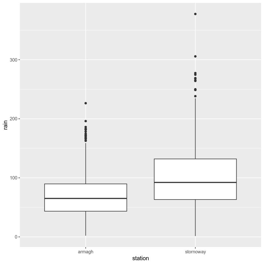
It does look like Stornoway Airport does get more rain, on average, than
Armagh. Using t.test(), we can test this hypothesis at the 99%
confidence level:
armagh.rain <- selected |>
    filter(station == 'armagh', !is.na(rain)) |> # select only rows where station == 'armagh'
    pull(rain) # select only the rain variable as a vector

stornoway.rain <- selected |>
    filter(station == 'stornoway', !is.na(rain)) |> # select only rows where station == 'stornoway'
    pull(rain) # select only the rain variable as a vector

# test whether mean(stornoway.rain) > mean(armagh.rain) at the 99% confidence interval
t.test(stornoway.rain, armagh.rain, alternative='greater', conf.level=0.99)
The output of t.test() tells us the data that we have used, the
value of the t statistic (22.877), the number of degrees of freedom
(df = 3075), and the p value of the test (p < 2.2e-16).
It also formulates the alternative hypothesis, gives us the 99% confidence interval for the difference in the means, and gives us the estimates of the mean value for each variable. Based on the results of the test, we can reject the null hypothesis, and conclude that Stornoway Airport does get more rain, on average, than Armagh.
Now, let’s look at an example of a one-sample t-test, to see if we can determine whether the mean of a small sample of summer temperatures provides a good estimate of the mean of all summer temperatures measured at Oxford.
First, we’ll select all of the summer values of tmax recorded at
Oxford, then calculate the mean value of these temperatures:
oxford_summer_tmax <- station_data |>
    filter(station == 'oxford', !is.na(tmax), season == 'summer') |> # select only rows where station == 'armagh'
    pull(tmax) # select only the tmax variable as a vector

# sample(30) # select a random sample of 50 values

mean(oxford_summer_tmax)
So the mean summer temperature measured in Oxford between 1853-2022 is
21.1°C - now, let’s take a random sample of 30 temperatures using
sample():
# select a random sample of 30 values
sample_tmax <- sample(oxford_summer_tmax, 30)
And finally, we conduct a one-sample t-test (two-sided), to see if our sample leads us to conclude whether the mean monthly maximum temperature is not equal to 21.1°C:
# test whether average summer monthly maximum temperature is not equal to 21.1
t.test(sample_tmax, mu=21.1, alternative='two.sided', conf.level=0.99)
non-parametric tests#
We can also conduct non-parametric hypothesis tests using R. The
example we will look at is the one- or two-sample Wilcoxon tests, using
wilcox.test()
(documentation). Let’s
start by looking at the Wilcoxon Rank Sum test, which is analogous to
the independent sample t-test. For this, we’ll use the same data that
we did before, again testing whether Stornoway Airport gets more
rainfall, on average, than Armagh:
# test whether mean(stornoway.rain) > mean(armagh.rain) at the 99% confidence interval
wilcox.test(stornoway.rain, armagh.rain, alternative='greater', conf.level=0.99)
analysis of variance#
Finally, we’ll see how we can set up and interpret an analysis of
variance test. In this example, we’ll only look at data from Armagh,
Oxford, and Stornoway Airport, because the Southampton time series ends
in 1999. We’ll first calculate the annually-averaged (or annual total)
values of tmax, tmin, and rain. Then, we’ll add a new
variable, period, to divide the observations into three different
50-year periods: 1871-1920, 1921-1970, and 1971-2020. Finally, we’ll
remove any remaining NA values, and assign this to a new object,
filtered_periods:
station_data |>
    filter(station %in% c('armagh', 'oxford', 'stornoway')) |> # select only armagh, oxford, and stornoway observations
    group_by(year) |>
    summarize(
        tmax = mean(tmax, na.rm = TRUE), # calculate the annually-averaged value of tmax
        tmin = mean(tmin, na.rm = TRUE), # calculate the annually-averaged value of tmin
        rain = sum(rain, na.rm = TRUE), # calculate the annual total rainfall
    ) |>
    mutate(
        period = case_when( # add a new variable, period, corre
            year %in% 1871:1920 ~ '1871-1920',
            year %in% 1921:1970 ~ '1921-1970',
            year %in% 1971:2020 ~ '1971-2020',
        )
    ) |>
    filter(!is.na(period)) -> filtered_periods # remove NA values and store in a new object
Before running the test, let’s make a box plot that shows the
distribution of tmax values among the three periods:
ggplot(data=filtered_periods, mapping=aes(x=period, y=tmax)) +
    geom_boxplot()
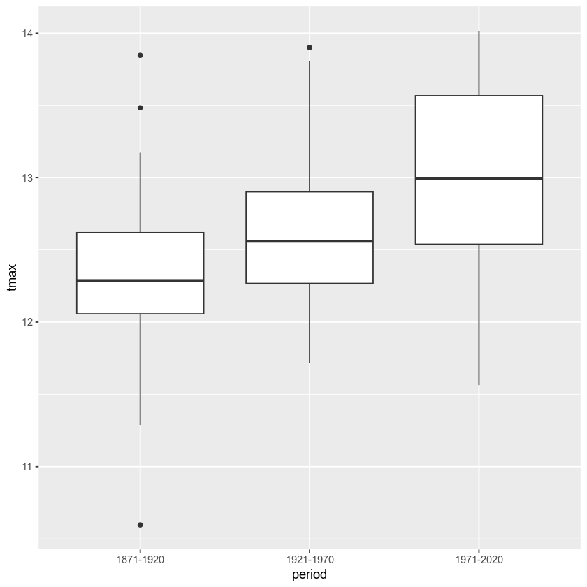
From this, it certainly appears as though there is a difference in the
mean value of tmax between the three periods. To formally test this,
we’ll use aov()
(documentation).
The first argument to aov() is a formula, as we discussed
earlier when looking at summary(). Here, we’re looking at a
two-sided formula, which has the form
response variable ~ explanatory variable(s). Here, we’re
investigating whether there is a relationship between value of
period and the value of tmax, which means that the formula
we use is tmax ~ period. We also need to make sure to pass the
filtered_periods object to the function using the data argument,
otherwise R won’t find the variables tmax and period:
tmax_aov <- aov(tmax~period, data=filtered_periods) # run aov on tmax as a function of period

tmax_aov # show the output of aov()
From this, we see the terms of the model - the sum of squares between groups (11.71181) and within groups (49.15164) in the top row, and the number of degrees of freedom between groups (2) and within groups (147) in the second row.
If we want to see the result of the test, we can summary() to show
the summary of the model:
summary(tmax_aov) # show the summary of the aov model
Here, we can see the significance value (Pr(>F)) is 1.51e-07, which
is also given a significance code of *** - meaning that there is a
significant difference between the groups at the 0.001 significance
level.
This doesn’t tell us which pairs of groups are different - for this, we
would need to run an additional test. As one example, we could use the
tmax_aov object, along with TukeyHSD()
(documentation), to compute
“Tukey’s Honest Significant Difference” between each pair of groups:
TukeyHSD(tmax_aov) # compute tukey's hsd using our aov model
From this, we can see the estimated difference in the means for each
pair of groups (diff), the lower (lwr) and upper (upr)
values of the 95% confidence interval of the difference, and the
adjusted p-value for each estimated difference. Using this, we can
clude that, at the 99% significance level, there is a significant
difference in tmax between the periods 1971-2020 and 1871-2020, and
between the periods 1971-2020 and 1921-1970.
exercise and next steps#
That’s all for this exercise. To help practice your skills, try at least one of the following:
Set up and run an AOV test to compare annual total rainfall at all four stations, using data from all avaialable years. Are there significant differences between the stations? Use
TukeyHSD()orpairwise.t.test()(documentation) to investigate further.Using only observations from Armagh, set up and run a test to see if there are significant differences in rainfall based on the season.
Using only observations from Oxford, is there a significant difference between the values of
tmaxin the spring and the autumn at the 99.9% confidence level?Using only observations from Stornoway Airport, is the value of tmin significantly lower in the winter, compared to the autumn?