linear regression using R#
Note
This is a non-interactive version of the exercise. If you want to run through the steps yourself and see the outputs, you’ll need to do one of the following:
follow the setup steps and work through the notebook on your own computer
open the workshop materials on binder and work through them online
open an R console or RStudio, copy the lines of code here, and paste them into the console to run them
In this exercise, we’ll see how we can use R for both simple and linear regression. We’ll also see how we can calculate the correlation between two variables, and get some additional practice working with grouped data.
data#
The data used in this exercise are the historic meteorological observations from the Armagh Observatory (1853-present), the Oxford Observatory (1853-present), the Southampton Observatory (1855-2000), and Stornoway Airport (1873-present), downloaded from the UK Met Office that we used in previous exercises.
getting started#
First, we’ll use library() to load the tidyverse package:
library(tidyverse)
next, we’ll use read_csv() to load the combined station data:
station_data <- read_csv(file.path('data', 'combined_stations.csv'))
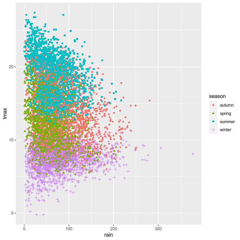
plotting relationships#
Before jumping into correlation and regreesion, let’s have a look at the
data we’re investigating. In the cell below, write some lines of code to
create a scatter plot of tmax vs rain, with different colors and
shapes for each season. Be sure to assign the plot to an object called
rain_tmax_plot:
# create a plot of tmax vs rain
# make a scatter plot with different colors and shapes, based on the season
rain_tmax_plot # show the plot
Now, use geom_smooth() to add a linear regression line to each group
- you should end up with four lines, colored according to the season:
# now add a geom_smooth to plot regression lines for each season
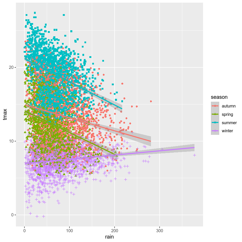
What kind of relationship is there between tmax and rain? Does
it depend on the season? How strong is the relationship, and what does
this mean for the slope of each regression line?
calculating correlation#
The next thing we’ll look at is how to calculate the correlation
between two variables, using cor()
(documentation). We’ll start by
calculating the covariance for all values of a variable, then use some
of the tools we’ve seen previously to calculate the correlation based on
different grouping variables.
for an entire dataset#
The basic use of cor() to calculate the correlation between two
variables x and y is cor(x, y). To calculate the correlation
between rain and tmax, then, we can use the $ operator to
select the rain and tmax variables. The use argument tells
R how to handle missing variables. In this case, we want to ignore
observations where either rain or tmax is missing - in other
words, we only want to use complete observations (complete.obs):
cor(station_data$rain, station_data$tmax, use='complete.obs') # calculate pearson's r for rain and tmax
by groups#
We’re more interested in calculating the correlation for different
groups - as you can see from the plots above, the relationship between
rain and tmax is not the same in each season - even though the
overall correlation is slightly negative, the correlation in winter is
clearly positive.
We’ve already seen all of the different parts we need here. To calculate
the correlation based on season, we can use group_by() to group
the dataset, then use summarize(), along with cor(), to
calculate the desired correlation.
By default, cor() calculates Pearson’s correlation, but we can also
calculate Spearman’s rho and Kendall’s tau coefficient:
corr_table <- station_data |>
    group_by(season) |> # group by season
    summarize(
        pearson = cor(rain, tmax, use='complete.obs'), # calculate pearson's r for rain and tmax
        spearman = cor(rain, tmax, use='complete.obs', method='spearman'), # calculate spearman's rho for rain and tmax
        kendall = cor(rain, tmax, use='complete.obs', method='kendall') # calculate kendall's tau for rain and tmax
    )

corr_table # show the table
simple linear regression#
We’ll start by fitting a linear model for spring. To prepare the data,
write a line of code below that selects only the spring observations,
and assigns the output to an object called spring:
# select only spring observations
To fit a linear model, we use the lm() function
(documentation). The first
argument for lm() is a formula representing the model to be fit.
Remember that a linear model with a single variable has the form:
where \(\beta\) is the intercept and \(\alpha\) is the slope of
the line. In R, the formula for this model is y ~ x -
remember that the response (dependent) variable is on the left side
of the ~ operator, and the explanatory (dependent) variable(s)
are on the right side of the operator. The coefficients \(\beta\)
and \(\alpha\) are implied in the form of the model, though we can
explicitly add an intercept (such as 0) to force the model to fit a
specific value.
So, the call to fit a linear relationship between tmax and rain
would look like this:
lm(tmax ~ rain, data=spring) # fit a linear model for tmax and rain, using spring data
The basic output of the model shows us the intercept (14.13683), and the
slope for rain (-0.02961). We can also use summary() to print
more information, once we assign the output of lm() to an object:
spring_lm <- lm(tmax ~ rain, data=spring) # fit a linear model for tmax and rain, using spring data

summary(spring_lm) # show the summary of the fit
The output of summary() shows quite a bit more information,
including the distribution of the residuals to the fit, the standard
error and p-value for the estimated coefficients, and the \(R^2\)
value.
If we want to extract the coefficients from the summary, we can use the
coef() (documentation)
built-in function on the output of summary():
coef(summary(spring_lm)) # extract the coefficients from the model summary
In this example, the output of coef() is a matrix, which is
similar to a data.frame. If we want to access the elements of the
matrix, we can use the extraction operators ([ and ]),
along with the row and column name of element we want. For example,
the following shows how to extract the estimate of the intercept from
the matrix:
spring_lm_coefs <- coef(summary(spring_mlm))

spring_lm_coefs["(Intercept)", "Estimate"] # get the estimate of the intercept
multiple linear regression#
Now, let’s try to fit a linear model of tmax with two variables:
rain and sun. Remember that multiple linear regression tries to
fit a model with the form:
With only two variables, this would look like:
And the corresponding formula in R looks like y ~ x_1 + x_2
(or tmax ~ rain + sun, using our variable names):
spring_mlm <- lm(tmax ~ rain + sun, data=spring) # fit a linear model for tmax and rain, using spring data

summary(spring_mlm) # show the summary of the fit
And we can extract the coefficients from the summary in the same way as before:
spring_mlm_coefs <- coef(summary(spring_mlm))

spring_mlm_coefs["rain", "Estimate"] # get the slope of the rain variable
bonus: linear regression with groups#
As a final exercise, let’s see how we can combine some of the tools we’ve used in the workshop so far, along with a few new ones, to fit linear models for each season without having to explicitly assign each selection to an object.
For this, we will use nest_by()
(documentation),
rather than group_by() - the idea is the same (group the table based
on different variables), but the output is different. Here, the ouptut
is a table with two (or more) columns: one column, data, which is a
nested table containing the data corresponding to the group, and
additional columns corresponding to the grouping variable(s).
Then, we can use mutate() create a column, model, that contains
the output of lm() applied to the data in each group. Finally, we
use list() (documentation) to
turn this output into a list so that it can be used in the table:
fits <- station_data |>
    nest_by(season) |> # create a nested table, grouped by season
    mutate(model = list(lm(tmax ~ rain, data = data))) # create a new variable, model, which is the output of the linear model

names(fits) # show the names of the columns
Now that we have this, we can use pull()
(documentation) to
extract this column as a list:
models <- fits |> pull(model) # extract the model column into a separate list

models # show the list
Note that each element of the list has a name that doesn’t tell us
any useful information ([[1]], [[2]], etc.) - ideally, we would
like to index the list using the name of each season. To do this, we can
use names() (documentation)
to assign the name of each season to the corresponding list element:
names(models) <- fits$season # assign the season name to each element of the list

models # show the object
Now, we can access the linear model for each season using its name - for example, to get the linear model for autumn:
models$autumn
And finally, we can use map() to apply the summary() function to
each element of the list, and assign the output of this to a new
object:
models |>
    map(summary) -> # use map to get the summary of each element of the list
    model_summary # assign the output to a new list object

coef(model_summary$autumn) # get the coefficients of the autumn linear model
exercise and next steps#
That’s all for this exercise, and for the exercises of this workshop. The next sessions are BYOD (“bring your own data”) sessions where you can start building your git project repository by applying the different concepts and skills that we have covered in the workshop. Before then, if you would like to practice these skills further, try at least one of the following suggestions:
Investigate the relationship between
tmaxandsunoverall, and by individual seasons, usingcor(). What kind of relationship do these variables appear to have? Remember to usedrop_na()to remove missing values!What is the relationship between
tminandsun? does it change by season?Set up and fit a multiple linear regression model for
air_frostas a function oftmax,tmin,sun, andrainin the winter. Which of these variables has the strongest effect onair_frost?