zonal statistics using rasterstats#

In this practical, we’ll see how we can combine vector and raster data for different analyses, including computing zonal statistics for a raster, and rasterizing a vector dataset.

The practical this week is provided as a Jupyter Notebook, which you can use to interactively work through the different steps of the practical.

getting started#

To get started with this week’s practical, you’ll need to first merge the week5 branch into the main branch, using one of the methods we’ve seen in previous weeks:

using GitHub Desktop [week2]
using the git command-line interface [week3]
using a Pull Request [week4]

Make sure that you have merged week5 into main using one of the methods outlined above before starting the practical.

The other thing you’ll need to do before starting this week’s practical is install a new python package, rasterstats, using conda via the command prompt.

Note

You can also install this package using Anaconda Navigator, as we did during the Week 4 SentinelSat exercise, but the following instructions are designed to give you some more experience using the conda CLI.

To do this, open the egm722 command prompt, then type the following command:

conda install -c conda-forge rasterstats

Press Enter. You should see something like the following (it may take a minute):

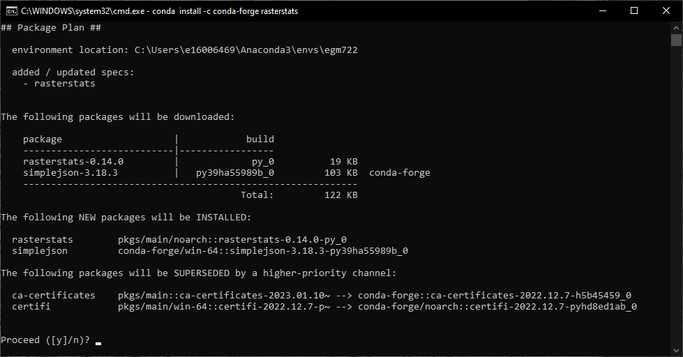
conda install running in the command prompt

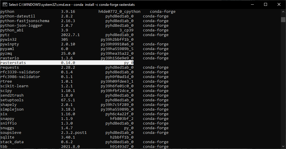
Type y and press Enter, and conda will install rasterstats into your current environment (egm722). Enter the following command:

conda list

You should see rasterstats included in the output of this command (you may need to scroll up to see it):

the output of conda list in the command prompt, showing that rasterstats is installed

At this point, you can launch Jupyter Notebooks from the command prompt, or from Anaconda Navigator, and begin to work through the notebook.

Note

Below this point is the non-interactive text of the notebook. To actually run the notebook, you’ll need to follow the instructions above to open the notebook and run it on your own computer!

Nick Cassavetes#

overview#

Up to now, we have worked with either vector data or raster data, but we haven’t really used them together. In this week’s practical, we’ll learn how we can combine these two data types, and see some examples of different analyses, such as zonal statistics or sampling raster data, that we can automate using python.

objectives#

learn how to use rasterstats to perform zonal statistics
use the zip built-in to combine iterables such as lists
learn how to handle exceptions using try … except blocks
rasterize polygon data using rasterio
learn how to mask and select (index) rasters using vector data
see additional plotting examples using matplotlib

data provided#

In the data_files folder, you should have the following: - LCM2015_Aggregate_100m.tif - NI_DEM.tif

getting started#

In this practical, we’ll look at a number of different GIS tasks related to working with both raster and vector data in python, as well as a few different python and programming concepts. To get started, run the cell below.

%matplotlib inline

import numpy as np
import rasterio as rio
import pandas as pd
import geopandas as gpd
import matplotlib.pyplot as plt
import rasterstats

zonal statistics#

In GIS, zonal statistics is a process whereby you calculate statistics for the pixels of a raster in different groups, or zones, defined by properties in another dataset. In this example, we’re going to use the Northern Ireland County border dataset from Week 2, along with a re-classified version of the Northern Ireland Land Cover Map 20151.

The Land Cover Map tells, for each pixel, what type of land cover is associated with a location - that is, whether it’s woodland (and what kind of woodland), grassland, urban or built-up areas, and so on. For our re-classified version of the dataset, we’re working with the aggregate class data, re-sampled to 100m resolution from the original 25m resolution.

The raster data type is unsigned integer with a bitdepth of 8 bits - that is, it has a range of possible values from 0 to 255. Even though it has this range of possible values, we only use 10 (11) of them:

Raster value	Aggregate class name
0	No Data
1	Broadleaf woodland
2	Coniferous woodland
3	Arable
4	Improved grassland
5	Semi-natural grassland
6	Mountain, heath, bog
7	Saltwater
8	Freshwater
9	Coastal
10	Built-up areas and gardens

In the cell below, we’ll first define a list of landcover class names, in the order shown in the table above. Then, we’ll use range() to create a list of values from 1 to 10, corresponding to the raster value of each landcover class.

# define the landcover class names in a list
names = ['Broadleaf woodland', 'Coniferous woodland', 'Arable', 'Improved grassland', 'Semi-natural grassland',
         'Mountain, heath, bog', 'Saltwater', 'Freshwater', 'Coastal', 'Built-up areas and gardens']

values = range(1, 11) # get numbers from 1-10, corresponding to the landcover values

Next, we’ll use a combination of the zip() built-in function (documentation), along with dict() (documentation), to create a dict object of key/value pairs that maps each raster value (the key) to a class name (the value):

landcover_names = dict(zip(values, names)) # create a dict of landcover value/name pairs

We’ll use this later on, when we want to make our outputs more readable/understandable.

In this part of the practical, we’ll try to work out the percentage of the entire country, and of each county individually, that is covered by each of these different landcovers.

To start, we’ll load the LCM2015_Aggregate_100m.tif raster, as well as the counties shapefile from Week 2:

# open the land cover raster and read the data
with rio.open('data_files/LCM2015_Aggregate_100m.tif') as dataset:
    xmin, ymin, xmax, ymax = dataset.bounds
    crs = dataset.crs
    landcover = dataset.read(1)
    affine_tfm = dataset.transform

# now, load the county dataset from the week 2 folder
counties = gpd.read_file('../Week2/data_files/Counties.shp').to_crs(crs)

Next, we’ll define a function that takes an array, and returns a dict object containing the count (number of pixels) for each of the unique values in the array:

def count_unique(array, names, nodata=0):
    '''
    Count the unique elements of an array.

    :param array: Input array
    :param names: a dict of key/value pairs that map raster values to a name
    :param nodata: nodata value to ignore in the counting

    :returns count_dict: a dictionary of unique values and counts
    '''
    count_dict = dict() # create the output dict
    for val in np.unique(array): # iterate over the unique values for the raster
        if val == nodata: # if the value is equal to our nodata value, move on to the next one
            continue
        count_dict[names[val]] = np.count_nonzero(array == val)
    return count_dict # return the now-populated output dict

Here, we have three input parameters: the first, array, is our array (or raster data). The next, names, is a dict of key/value pairs to provide human-readable names for each raster value. Finally, nodata is the value of the input array that we should ignore.

The first line of the function defines an empty dict:

count_dict = dict()

This is the empty container into which we’ll place the key/value pairs corresponding to the count for each landcover class.

Next, using numpy.unique() (documentation), we get an array containing the unique values of the input array.

Note that this works for data like this raster, where we have a limited number of pre-defined values. For something like a digital elevation model, which represents continuous floating-point values, we wouldn’t want to use this approach to bin the data - we’ll see how we can handle continuous data later on.

For each of the different unique values val, we find all of the locations in array that have that value (array == val). Note that this is actually a boolean array, with values of either True where array == val, and False where array != val. numpy.count_nonzero() (documentation) then counts the number of non-zero (in this case, True) values in the array - that is, this:

np.count_nonzero(array == val)

tells us the number of pixels in array that are equal to val. We then assign this to our dictionary with a key that is a str representation of the value, before returning our count_dict variable at the end of the function.

Run the cell below to run the function on our landcover raster:

landcover_count = count_unique(landcover, landcover_names)
print(landcover_count) # show the results

Exercise: can you work out the percentage area of Northern Ireland that is covered by each of the 10 landcover classes?

# start by using count_unique to get the number of pixels corresponding to each landcover class

# now, get the total number of pixels in the image that aren't nodata
# hint: use np.count_nonzero()

# now, iterate over the dictionary items to express the number of pixels as a percentage of the total pixels

Now, let’s have a look at the help for rasterstats.gen_zonal_stats() (documentation), which will tell us how we can use rasterstats to get zonal statistics for a raster and vector geometry:

help(rasterstats.gen_zonal_stats)

In the output of the cell above, you should see the usage for rasterstats.gen_zonal_stats(), which is the same as the usage for rasterstats.zonal_stats(). Have a look at the documentation - we’ll go over an example below, but there are many more useful features that we won’t go into in the tutorial.

In the following cell, we use rasterstats.zonal_stats() (documentation) with our counties and landcover datasets to do the same exercise as above (counting unique pixel values).

Rather than counting the pixels in the entire raster, however, we want to count the number of pixels with each land cover value that fall within a specific area defined by each of the features in the counties dataset:

county_stats = rasterstats.zonal_stats(counties, # the shapefile to use
                                       landcover, # the raster to use - here, we're using the numpy array loaded using rasterio
                                       affine=affine_tfm, # the geotransform for the raster
                                       categorical=True, # whether the data are categorical
                                       category_map=landcover_names,
                                       nodata=0 # the nodata value for the raster
                                      )

print(type(county_stats)) # county_stats is a list of dict objects
print(county_stats[0]) # shows the landcover use for county tyrone (index 0 in counties geodataframe)

the zip built-in#

We introduced the zip() built-in function above, but it’s worth discussing this powerful and useful function in a bit more detail.

In Python 3, zip() returns a zip object that combines elements from each of the iterable objects passed as arguments:

x = [1, 2, 3, 4]
y = ['a', 'b', 'c', 'd']

print(zip(x, y))

We have seen something similar with iterator objects before - for example, the output of range() is an iterator. As we have seen, we can iterate over the items of the iterator object, or we can use something like list() to convert the iterator into another type of object:

print(list(zip(x, y)))

And, as we saw above, we can also pass the output of zip() to dict(), to create a dict of key/value pairs - this is an efficient way to create a dict object from two list objects of different items:

print(dict(zip(x, y)))

One thing to keep in mind, though, is that with zip(x, y), each of the elements of x is paired with the corresponding element from y. If x and y are different lengths, zip(x, y) will only use up to the shorter of the two:

x = [1, 2, 3]

list(zip(x, y))

As a final example, we can also use zip() to combine more than two iterables - we’re not limited to a single pair of iterables:

x = [1, 2, 3, 4]
y = ['a', 'b', 'c', 'd']
z = ['i', 'ii', 'iii', 'iv']

print(list(zip(x, y, z)))

Now, let’s use zip() to create a dict that returns the landcover stats for each county, given the county name.

First, we can use a list comprehension to get a list of the county names, formatted using str.title():

names = [n.title() for n in counties['CountyName']] # use str.title() because we're not shouting

Now, we use dict() and zip() to create the dict object of landcover stats by county:

county_dict = dict(zip(names, county_stats))
print(county_dict['Tyrone']) # should be the same output as before

handling Exceptions with try … except#

Now, let’s add information about the percent landcover to the counties table. We’ll start by using creating a dict that takes the full landcover class name, and shortens it so that it can be used as a column header:

short_names = ['broadleaf', 'coniferous', 'arable', 'imp_grass', 'nat_grass',
               'mountain', 'saltwater', 'freshwater', 'coastal', 'built_up']
short_dict = dict(zip(landcover_names.values(), short_names)) # use dict and zip with the full names

Now, we can use this to populate the data table with new columns for each landcover class:

for ind, row in counties.iterrows(): # use iterrows to iterate over the rows of the table
    county_data = county_dict[row['CountyName'].title()] # get the landcover data for this county
    for name in landcover_names.values(): # iterate over each of the landcover class names
        counties.loc[ind, short_dict[name]] = county_data[name] # add the landcover count to a new column

What happened here?

From the error message above, we can see that there is no entry for Saltwater in the data for this county (Tyrone):

print(row['CountyName'].title()) # show the county name that caused the error
print('Saltwater' in county_dict[row['CountyName'].title()].keys()) # is Saltwater a valid key for this county?

Because Saltwater is not in the list of key values for this dict, when we try to use Saltwater as a key in the county_data dictionary, it raises a KeyError.

The problem that we have here is that we don’t necessarily have all landcover classes represented in every county. We shouldn’t expect to, either - County Tyrone is an inland county, so it makes sense that it wouldn’t have any saltwater areas.

One way to handle this could be to insert an if/else block to check that the landcover class is present in the dict before trying to access it. This would check whether the value of name is a key of county_data - if it isn’t, then it will add a value of 0 to the table for that column:

for ind, row in counties.iterrows(): # use iterrows to iterate over the rows of the table
    county_data = county_dict[row['CountyName'].title()] # get the landcover data for this county
    for name in landcover_names.values(): # iterate over each of the landcover class names
        if name in county_data.keys(): # check that name is a key of county_data
            counties.loc[ind, short_dict[name]] = county_data[name] # add the landcover count to a new column
        else:
            counties.loc[ind, short_dict[name]] = 0 # if name is not present, value should be 0.

Another option is to use a `try … except <https://realpython.com/python-exceptions/#the-try-and-except-block-handling-exceptions>`__ block to “catch” and handle an exception:

try:
    # run some code
except:
    # run this if the try block causes an exception

In general, it’s not recommended to just have a bare except: clause, as this will make it harder to interrupt a program. In our specific case, we only want the interpreter to ignore KeyError exceptions - if there are other problems, we still need to know about those.

In our example, the try … except block looks like this:

for ind, row in counties.iterrows(): # use iterrows to iterate over the rows of the table
    county_data = county_dict[row['CountyName'].title()] # get the landcover data for this county
    for name in landcover_names.values(): # iterate over each of the landcover class names
        try:
            counties.loc[ind, short_dict[name]] = county_data[name] # add the landcover count to a new column
        except KeyError: # we can ignore KeyErrors, because this just means the landcover class has a value of 0
            counties.loc[ind, short_dict[name]] = 0 # if name is not present, value should be 0.

counties # just to show the table in the output below

Now, we can see that the table has had an additional 10 columns added (one for each landcover class), with each column being filled with the number of pixels in each county that are classified as that landcover class.

As one final step, let’s update the table so that the value corresponds to the percentage of each county’s area covered by each landcover class:

for ind, row in counties.iterrows(): # iterate over the rows of the table
    counties.loc[ind, short_names] = 100 * row[short_names] / row[short_names].sum()
counties # just to show the table in the output below

In the above, you can see that we’ve indexed the table using the list of column names short_name, which ensures that we only select the columns we’re interested in.

Looking at the table above, what landcover class dominates each county? Does this make sense, given what you know about Northern Ireland?

As a final exercise, modify the cell below so that each cell represents the total area (in square km) covered by each landcover class, rather than the number of pixels or the percent area of each county.

As a small hint, you should only need to change a single line:

for ind, row in counties.iterrows(): # use iterrows to iterate over the rows of the table
    county_data = county_dict[row['CountyName'].title()] # get the landcover data for this county
    for name in landcover_names.values(): # iterate over each of the landcover class names
        try:
            counties.loc[ind, short_dict[name]] = county_data[name] # add the landcover count to a new column
        except KeyError:
            counties.loc[ind, short_dict[name]] = 0 # if name is not present, value should be 0.

counties # just to show the table in the output below

rasterizing vector data using rasterio#

rasterstats provides a nice tool for quickly and easily extracting zonal statistics from a raster using vector data. Sometimes, though, we might want to rasterize our vector data - for example, in order to mask our raster data, or to be able to select pixels. To do this, we can use the rasterio.features module (documentation):

import rasterio.features # we have imported rasterio as rio, so this will be rio.features (and rasterio.features)

rasterio.featureshas a number of different methods, but the one we are interested in here is rasterize() (documentation):

help(rio.features.rasterize)

Here, we pass an iterable object (list, tuple, array, etc.) that contains (geometry, value) pairs. value determines the pixel values in the output raster that the geometry overlaps. If we don’t provide a value, it takes the default_value or the fill value.

So, to create a rasterized version of our county outlines, we could do the following:

shapes = list(zip(counties['geometry'], counties['COUNTY_ID'])) # get a list of geometry, value pairs
county_mask = rio.features.rasterize(shapes=shapes, # the list of geometry/value pairs
                                     fill=0, # the value to use for cells not covered by any geometry
                                     out_shape=landcover.shape, # the shape of the new raster
                                     transform=affine_tfm) # the geotransform of the new raster

The first line uses zip() and list() to create a list of (geometry, value) pairs, and the second line actually creates the rasterized array, county_mask.

Note that in the call to rasterio.features.rasterize(), we have to set the output shape (out_shape) of the raster, as well as the transform - that is, how we go from pixel coordinates in the array to real-world coordinates.

Since we want to use this rasterized output with our landcover, we use the shape of the landcover raster, as well as its transform (affine_tfm) - that way, the outputs will line up as we expect.

The cell below will display the county_mask raster in a matplotlib Figure:

fig, ax = plt.subplots(1, 1)
im = ax.imshow(county_mask) # visualize the rasterized output
fig.colorbar(im) # show a colorbar

As you can see, this provides us with an array whose values correspond to the COUNTY_ID of the county feature at that location (check the counties GeoDataFrame again to see which county corresponds to which ID). In the next section, we’ll see how we can use arrays like this to investigate our data further.

masking and indexing rasters#

So far, we’ve seen how we can index an array (or a list, a tuple, …) using simple indexing (e.g., myList[0]) or slicing (e.g., myList[2:4]). numpy arrays, however, can actually be indexed using other arrays of type bool (the elements of the array are boolean (True/False) values) - similar to how we have used conditional statements to select rows from a GeoDataFrame.

In this section, we’ll see how we can use this, along with our rasterized vectors, to select and investigate values from a raster using boolean indexing.

To start, we’ll open our dem raster - note that this raster has the same georeferencing information as our landcover raster, so we don’t have to load all of that information, just the raster band:

with rio.open('data_files/NI_DEM.tif') as dataset:
    dem = dataset.read(1)

From the previous section, we have an array with values corresponding each of the counties of Northern Ireland. Using numpy, we can use this array to select elements of other rasters by creating a mask, or a boolean array - that is, an array with values of True and False. For example, we can create a mask corresponding to County Antrim (COUNTY_ID=1) like this:

county_antrim = county_mask == 1

Let’s see what this mask looks like:

county_antrim = county_mask == 1

fig, ax = plt.subplots(1, 1)
ax.imshow(county_antrim) # visualize the rasterized output

We can also combine expressions using functions like `np.logical_and() <https://numpy.org/doc/stable/reference/generated/numpy.logical_and.html>`__ or `np.logical_or() <https://numpy.org/doc/stable/reference/generated/numpy.logical_or.html>`__. If we wanted to create a mask corresponding to both County Antrim (county_mask == 3) and County Down (county_mask == 1), we could do the following:

antrim_and_down = np.logical_or(county_mask == 3, county_mask == 1)

fig, ax = plt.subplots(1, 1)
ax.imshow(antrim_and_down)

We could then find the mean elevation of these two counties by indexing, or selecting, pixels from dem using our mask:

ad_elevation = dem[antrim_and_down] # index the array using the antrim_and_down mask
print('Mean elevation: {:.2f} m'.format(ad_elevation.mean()))

Now let’s say we wanted to investigate the two types of woodland we have, broadleaf and conifer. One thing we might want to look at is the area-elevation distribution of each type. To do this, we first have to select the pixels from the DEM that correspond to the broadleaf woodlands, and all of the pixels corresponding to conifer woodlands:

broad_els = dem[landcover == 1] # get all dem values where landcover = 1
conif_els = dem[landcover == 2] # get all dem values where landcover = 2

Now, we have two different arrays, broad_els and conif_els, each corresponding to the DEM pixel values of each landcover type. We can plot a histogram of these arrays using plt.hist() (documentation), but this will only tell us the number of pixels - to work with areas, remember that we have to convert the pixel counts into areas by multiplying with the pixel area (here, 100 m x 100 m).

First, though, we can use numpy.histogram() (documentation), along with an array representing our elevation bins, to produce a count of the number of pixels with an elevation that falls within each bin. We’ll use numpy.arange() (documentation) to generate an array of elevation bins ranging from 0 to 600 meters, spaced by 5 meters:

el_bins = np.arange(0, 600, 5) # create an array of values ranging from 0 to 600, spaced by 5.

broad_count, _ = np.histogram(broad_els, el_bins) # bin the broadleaf elevations using the elevation bins
conif_count, _ = np.histogram(conif_els, el_bins) # bin the conifer elevations using the elevation bins

broad_area = broad_count * 100 * 100 # convert the pixel counts to an area by multipling by the pixel size in x, y
conif_area = conif_count * 100 * 100

Finally, we can plot the area-elevation distribution for each land cover type using plt.bar() (documentation):

fig, ax = plt.subplots(1, 1, figsize=(8, 8)) # create a new figure and axes object

# plot the area-elevation distributions using matplotlib.pyplot.bar(), converting from sq m to sq km:
_ = ax.bar(el_bins[:-1], broad_area / 1e6, align='edge', width=5, alpha=0.8, label='Broadleaf Woodland')
_ = ax.bar(el_bins[:-1], conif_area / 1e6, align='edge', width=5, alpha=0.8, label='Conifer Woodland')

ax.set_xlim(0, 550) # set the x limits of the plot
ax.set_ylim(0, 30) # set the y limits of the plot

ax.set_xlabel('Elevation (m)') # add an x label
ax.set_ylabel('Area (km$^2$)') # add a y label
ax.legend() # add a legend

From this, we can clearly see that Conifer woodlands tend to be found at much higher elevations than Broadleaf woodlands, and at a much larger range of elevations (0-500 m, compared to 0-250 m or so).

With these samples (broad_els, conif_els), we can also calculate statistics for each of these samples using numpy functions such as np.mean() (documentation), np.median() (documentation), np.std() (documentation), and so on:

print('Broadleaf mean elevation: {:.2f} m'.format(np.mean(broad_els)))
print('Broadleaf median elevation: {:.2f} m'.format(np.median(broad_els)))

Of the 10 different landcover types shown here, which one has the highest mean elevation? What about the largest spread in elevation values?

Starting from the initial code in the cell below, create a DataFrame of descriptive statistics of the elevation for each landcover type, which will help you answer this question.

# create a new pandas DataFrame with 6 columns
landcover_els = pd.DataFrame(columns=['name', 'mean', 'median', 'std. dev', 'max', 'min', 'range'])

landcover_els['name'] = short_names # add the short names to the 'name' column

# now, write a loop that will populate the table with descriptive statistics about the elevation
# of each landcover class

Next steps#

That’s all for this practical. In lieu of an additional exercise this week, spend some time working on your project - are there concepts or examples from this practical that you can incorporate into your project?

Footnotes#

1Rowland, C.S.; Morton, R.D.; Carrasco, L.; McShane, G.; O’Neil, A.W.; Wood, C.M. (2017). Land Cover Map 2015 (25m raster, N. Ireland). NERC Environmental Information Data Centre. doi:10.5285/47f053a0-e34f-4534-a843-76f0a0998a2f

zonal statistics using rasterstats

Contents

zonal statistics using rasterstats#

getting started#

Nick Cassavetes#

overview#

objectives#

data provided#

getting started#

zonal statistics#

the zip built-in#

handling Exceptions with try … except#

rasterizing vector data using rasterio#

masking and indexing rasters#

Next steps#

Footnotes#