change vector analysis#
Tip
The script for this tutorial can be found via this direct link.
Alternatively, if you have already added the repository, you can open the script from the Code Editor, by
navigating to 03_change_detection/04_change_vectors.js under the Reader section.
For this tutorial, we’ll use the same images that we used for previous tutorials on change detection – this time, using change vector analysis (CVA). While CVA can be used for any number of band differences, we’re going to stick to the differences in NIR and Red reflectance between the two images. Sticking with only two bands helps us visualize the changes in two dimensions - once we start adding more bands (dimensions), it becomes more difficult to visualize.
preparation#
Because we are working with sensors that have different band names, we must first re-name the bands so that when we
subtract them, the correct bands are paired together. First, we do this for the before image, using both
ee.Image.select() to select only the bands of interest, and ee.Image.rename()
(documentation) to rename the bands:
// select only the bands we're interested in, then rename to match OLI
before = before
          .select(['SR_B1', 'SR_B2', 'SR_B3', 'SR_B4', 'SR_B5', 'SR_B7'])
          .rename(['SR_B2', 'SR_B3', 'SR_B4', 'SR_B5', 'SR_B6', 'SR_B7']);
Warning
If we don’t do this step, the result of using ee.Image.subtract() will have OLI Band 2 (Blue) paired with
TM Band 2 (Green), OLI Band 3 (Green) paired with TM Band 3 (Red), and so on.
Because ee.Image.subtract() requires that the images have the same number of bands, we need to also select
the relevant bands from the after image:
// select only the bands we're interested in
after = after.select(['SR_B[2-7]']);
calculating change vectors#
The rest of this script is used to calculate the magnitudes and angles of the change vectors, starting with the difference between the 1986 and 2022 images:
// compute the difference between the two images, and select bands 7 and 6 (SWIR2 and SWIR1)
var diff = after.subtract(before).select(['SR_B7', 'SR_B6']);
Note
When we use ee.Image.subtract(), the result subtracts each band of the second image from the same band of
the first image (assuming that they share band names). So, in this line of code:
var diff = after.subtract(before)
We would get back an image with the difference of all of the bands that after and before share in common.
By selecting only SR_B7 and SR_B6, however, we end up with just the difference in those two bands.
Next, we calculate the magnitudes of the change vectors. First, we use ee.Image.pow()
(documentation) to square each of the input bands,
then use ee.Image.reduce() (documentation)
along with ee.Reducer.sum() (documentation)
and ee.Reducer.unweighted() (documentation)
to get the sum of each of the squares. Next, we use ee.Image.sqrt()
(documentation) to take the square root of the
sum of the squares, before finally using ee.Image.rename() to rename this band magnitude:
// compute the magnitude of the change vectors as the square root of the
// sum of the squared differences.
var magnitude = diff.pow(2).reduce(ee.Reducer.sum().unweighted())
  .sqrt().rename('magnitude');
To get the angle of each change vector (converted from radians to degrees). we use ee.Image.atan2()
(documentation), then use
ee.Image.multiply() and ee.Image.divide() to convert the output from radians to degrees:
// compute the angle of the change vectors and convert to degrees
var angle = diff.select('SR_B6').atan2(diff.select('SR_B7'))
  .multiply(180).divide(Math.PI).rename('angle');
Finally, we reclassify the angles so that the values in the image correspond to the quadrant the angle
falls in. For this, we use ee.Image.where()
(documentation):
// create a reclassified image of the angles, with the value set to the quadrant
// each angle range corresponds to.
var angleReclass = ee.Image(1)
          .where(angle.gt(0).and(angle.lte(90)), 1)
          .where(angle.gt(90).and(angle.lte(180)), 2)
          .where(angle.gt(-180).and(angle.lte(-90)), 3)
          .where(angle.gt(-90).and(angle.lte(0)), 4).clip(boundary);
Here, angles between 0 and 90 degrees get a value of 1; between 90 and 180 degrees, a value of 2, between -180
and -90 (or 180 and 270 degrees3) a value of 3, and finally between -90 and 0 (or 270 and 360), a value of
4.
Next, we use ee.Image.updateMask() (documentation)
mask the reclassified image so that only “large enough” changes (magnitude \(\geq\) 0.06) are shown:
// threshold the reclass image by changes w/ magnitude greater than 0.06
angleReclass = angleReclass.updateMask(magnitude.gte(0.06));
interpreting changes#
Run the script, then toggle the reclass angle layer on:
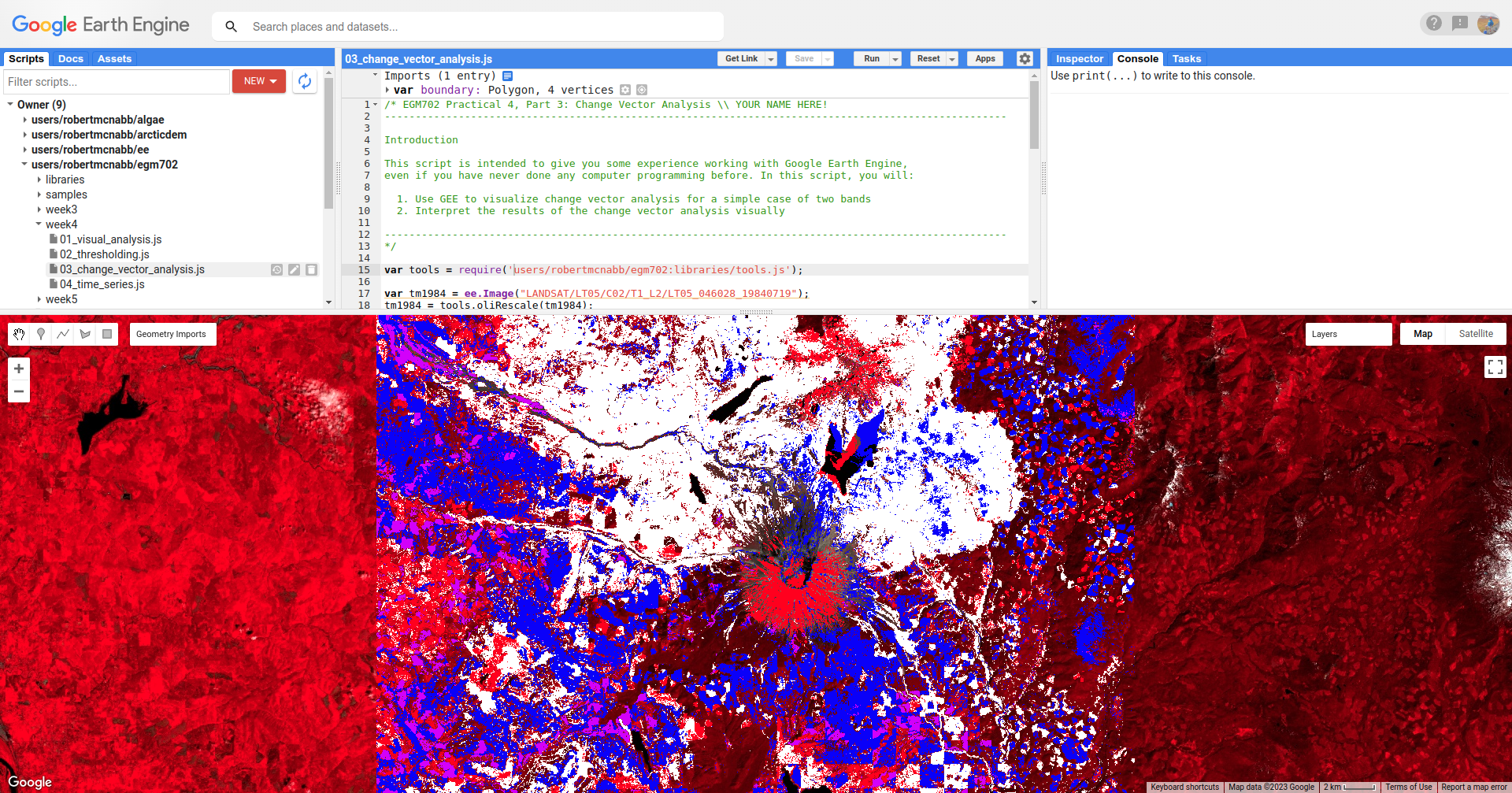
In this image, red colors correspond to increases in both SWIR1 and SWIR2 reflectance, white corresponds to
increases in SWIR2 and decreases in SWIR1 reflectance, purple corresponds to decreases in SWIR2 and increases in SWIR1
reflectance, and blue corresponds to decreases in both SWIR2 and SWIR1 reflectance.
You can also consult the diagram shown below:
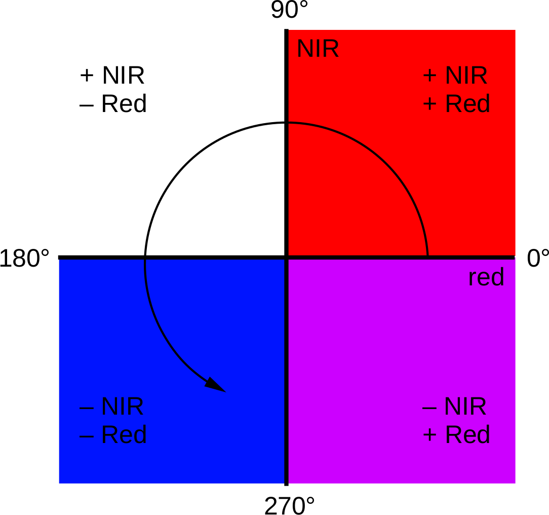
For the most part, the red color represents pixels where natural surfaces such as vegetation or water have been
replaced by built environments - this is particularly noticeable around the Zhujiang River Estuary, where large areas of
land fill have changed the shoreline dramatically.
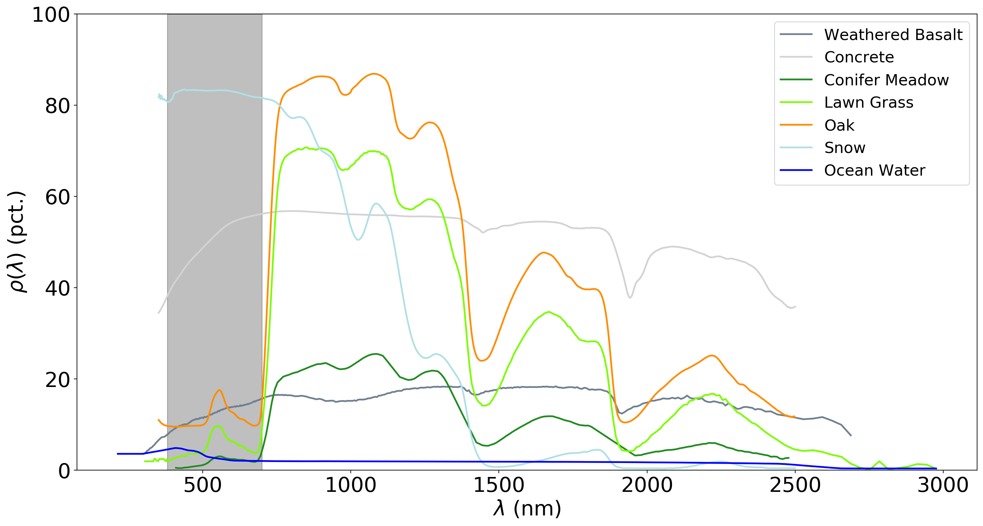
In a number of areas, the blue color represents forest growth. To understand why this is, we have to remember both what these changes represent – a decrease in both Red and NIR reflectance – and also what the forest is replacing: in many cases, grassy meadows or new-growth trees, both of which tend to have higher spectral reflectance than conifer forests:
Question
Using the diagram above and the colors on the map, what other differences do you notice?
Remember that some differences (or changes) might represent more than one kind of surface change. All we can tell by looking at the reclassified angle map is the broad direction of the change; we need to do a bit more to be able to explain what we see in terms of the physical changes that have taken place.
next steps#
In the 03_change_vector_analysis.js script, try changing the number of classes from 4 to 8 by copying and pasting
the following code at the end of the script, then re-running the script:
// re-classify the angles into 8 classes
var angleReclass2 = ee.Image(1)
          .where(angle.gt(0).and(angle.lte(45)), 1)
          .where(angle.gt(45).and(angle.lte(90)), 2)
          .where(angle.gt(90).and(angle.lte(135)), 3)
          .where(angle.gt(135).and(angle.lte(180)), 4)
          .where(angle.gt(-180).and(angle.lte(-135)), 5)
          .where(angle.gt(-135).and(angle.lte(-90)), 6)
          .where(angle.gt(-90).and(angle.lte(-45)), 7)
          .where(angle.gt(-45).and(angle.lte(0)), 8).clip(boundary);

// threshold the reclass image by changes w/ magnitude greater than 0.06
angleReclass2 = angleReclass2.updateMask(magnitude.gte(0.06));

// use an 8 color palette to visualize this color map
Map.addLayer(angleReclass2, {palette: ['b35806', 'e08214', 'fdb863', 'fee0b6',
  'd8daeb', 'b2abd2', '8073ac', '542788']}, 'reclass angle - 8 classes', true);
How does this compare to the 4 class visualization? Consider the following questions:
Look at the areas of clear-cut forest to the NE of the mountain. Do you notice differences between different patches, or within individual patches, that aren’t apparent in the 4 class image?
Pay attention to the differences between angle class 3 (angles between 90 and 135 degrees) and angle class 4 (angles between 135 and 180 degrees). These correspond to increases in NIR reflectance, and decreases in red reflectance; angle class 3 represents smaller decreases in red reflectance, while angle class 4 represents larger decreases. Using the angle change map and the original false color composites, what kind of changes are you able to discern here?
notes and references#
- 3
The reason that we use -180 and -90 here, instead of 180 and 270 (or -90 and 0 instead of 270 and 360) is because the output of
ee.Image.atan2()returns values between \(-\pi\) (-180 \(^\circ\)) and \(+\pi\) (180 \(^\circ\)).