linear regression using python#
Note
This is a non-interactive version of the exercise. If you want to run through the steps yourself and see the outputs, you’ll need to do one of the following:
follow the setup steps and work through the notebook on your own computer
open the workshop materials on binder and work through them online
open a python console, copy the lines of code here, and paste them into the console to run them
In this exercise, we’ll see how we can use python for both simple and linear regression. We’ll also see how we can calculate the correlation between two variables, and get some additional practice working with grouped data.
data#
The data used in this exercise are the historic meteorological observations from the Armagh Observatory (1853-present), the Oxford Observatory (1853-present), the Southampton Observatory (1855-2000), and Stornoway Airport (1873-present), downloaded from the UK Met Office that we used in previous exercises.
getting started#
First, we’ll import the various packages that we will be using here:
pandas, for reading the data from a file;
seaborn, for plotting the data;
scipy.stats, for calculating correlation coefficients;
pingouin, for linear regression;
pathlib, for working with filesystem paths.
import pandas as pd
import seaborn as sns
from scipy import stats
import pingouin as pg
from pathlib import Path
Next, we’ll use pd.read_csv() to load the combined station data:
station_data = pd.read_csv(Path('data', 'combined_stations.csv'), parse_dates=['date']) # load the combined station data
plotting relationships#
Before jumping into correlation and regreesion, let’s have a look at the
data we’re investigating. In the cell below, write some lines of code to
create a scatter plot of tmax vs rain, with different colors,
shapes, and a regression line for each season. Be sure to assign the
plot to an object called rain_tmax_plot:
# your code goes here!
rain_tmax_plot # show the plot
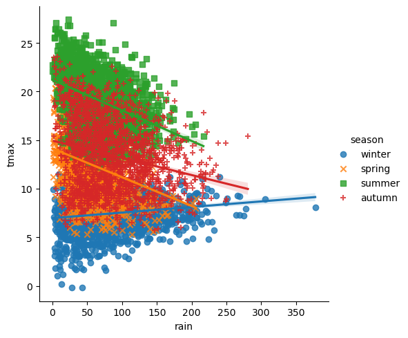
What kind of relationship is there between tmax and rain? Does
it depend on the season? How strong is the relationship, and what does
this mean for the slope of each regression line?
calculating correlation#
The next thing we’ll look at is how to calculate the correlation
between two variables, using a few different methods. We’ll start by
calculating the covariance for all values of a variable in a
DataFrame, then we’ll have a look at calculating correlation using
scipy.stats
(documentation).
using pandas .corr()#
The basic use of corr()
(documentation)
calculates Pearson’s correlation coefficient between each column in the
table, pairwise. With the method argument, we can also calculate
Spearman’s rho (method='spearman') and Kendall’s tau
(method='kendall').
Because we have non-numeric variables in the table, we’ll use the
numeric_only argument to avoid a ValueError being raised.
Helpfully, .corr() ignores any NaN values for us, so we don’t
have to
station_data.corr(numeric_only=True) # calculate the correlation between all numeric variables in the table
Out of all of the variables in the table, which have the strongest correlation (ignoring the values on the diagonal)? Does this make sense?
by groups#
We’re more interested in calculating the correlation for different
groups - as you can see from the plot above, the relationship between
rain and tmax is not the same in each season - even though the
overall correlation is slightly negative, the correlation in winter is
clearly positive.
We’ve already seen all of the different parts we need here. To calculate
the correlation based on season, we can use .groupby() to group
the dataset before calling .corr():
station_data.groupby('season')[['rain', 'tmax']].corr() # calculate pearson's r for rain and tmax, grouped by season
using scipy.stats#
From the outputs above, you can see that pandas.DataFrame.corr()
outputs the full covariance matrix, not just the correlation value we’re
interested in. In the cells below, we’ll see how we can use some of what
we have learned previously, along with scipy.stats, to create a
DataFrame with just the correlation values between rain and
tmax.
In the cell below, we’ll use a for loop to calculate correlation
coefficients (Pearson’s r, Spearman’s rho, and Kendall’s tau) for
rain and tmax based on data from each season. We’ll build a
nested list of the correlation coefficients for each season by first
creating an empty list, then using list.append() to add the
coefficients for each season in turn.
Before running the cell, be sure to create an object, seasons, that
contains the names of each season. You can write this explicitly, but
you might want to practice getting this output from the data directly.
# get a list of season names - remember that there's more than one way to do this!
corr_data = [] # initalize an empty list

for season in seasons:
    season_data = station_data.loc[station_data['season'] == season].dropna(subset=['rain', 'tmax']) # select the data for this season, drop nan values from rain and tmax
    this_corr = [stats.pearsonr(season_data['rain'], season_data['tmax']).statistic, # calculate pearson's r between rain and tmax
                 stats.spearmanr(season_data['rain'], season_data['tmax']).statistic, # calculate spearman's rho between rain and tmax
                 stats.kendalltau(season_data['rain'], season_data['tmax']).statistic] # calculate kendall's tau between rain and tmax
    corr_data.append(this_corr) # add these values to the list

corr_data # show the nested list of correlation values
Now that we have created the nested list (effectively, an array of
values), we can create a new DataFrame object by specifying the
data, index, and columns arguments:
corr_df = pd.DataFrame(data=corr_data, index=seasons, columns=['pearson', 'spearman', 'kendall']) # create a dataframe with the correlation data
corr_df # show the correlation dataframe
Note that calculating the correlation coefficient using scipy.stats
has an additional benefit - unlike with pandas.DataFrame.corr(),
scipy.stats will also provide a significance value for the
calculated correlation:
corr = stats.pearsonr(station_data.dropna(subset=['rain', 'tmax'])['rain'],
                      station_data.dropna(subset=['rain', 'tmax'])['tmax'])

print(f"calculated value of r: {corr.statistic:.3f}")
print(f"calculated p-value of r: {corr.pvalue}")
And, using pg.corr()
(documentation)
gives us even more information, such as the confidence interval for the
correlation value, as well as additional options for calculating the
correlation coefficient:
# calculate the biweight midcorrelation between rain and tmax
pg.corr(station_data.dropna(subset=['rain', 'tmax'])['rain'],
        station_data.dropna(subset=['rain', 'tmax'])['tmax'], method='bicor')
simple linear regression#
We’ll start by fitting a linear model for spring. To prepare the data,
write a line of code below that selects only the spring observations,
and assigns the output to an object called spring:
# select only spring observations
Remember that a linear model with a single variable has the form:
where \(\beta\) is the intercept and \(\alpha\) is the slope of
the line. To fit a linear model using pingouin, we use
pg.linear_regression()
(documentation).
The main inputs to pg.linear_regression() are X, the
observations of the explanatory (independent) variable(s), and
y, the observations of the response (dependent) variables. We
can also specify the significance level (alpha) to use when
calculating the statistics of the fitted model, as well as additional
arguments. By default, pg.linear_regression() adds an intercept to
be fitted.
So, the process to fit a linear relationship between tmax and
rain would look like this:
xdata = spring.dropna(subset=['rain', 'tmax'])['rain'] # select the rain variable, after dropping NaN values
ydata = spring.dropna(subset=['rain', 'tmax'])['tmax'] # select the tmax variable, after dropping NaN values

lin_model = pg.linear_regression(xdata, ydata, alpha=0.01) # run the regression at the 99% significance level

lin_model.round(3) # round the output table to 3 decimal places
The output of pg.linear_regression() is a DataFrame with the
following columns:
names: the names of the outputs (intercept) and the slope for each explanatory variable;coef: the values of the regression coefficients;se: the standard error of the estimated coefficients;T: the t-statistic of the estimates;pval: the p-values of the t-statistics;r2: the coefficient of determination;adj_r2: the adjusted coefficient of determination;CI{alpha/2}%: the lower value of the confidence interval;CI{1-alpha/2}%: the upper value of the confidence interval;relimp: the relative contribution of each predictor to the final (ifrelimp=True);relimp_perc: the percent relative contribution
The ouptut DataFrame also has hidden attributes such as the
residuals (lin_model.residuals_), the degrees of freedom of the
model (lin_model.df_model_), and the degrees of freedom of the
residuals (lin_model.df_resid_).
multiple linear regression#
Now, let’s try to fit a linear model of tmax with two variables:
rain and sun. Remember that multiple linear regression tries to
fit a model with the form:
With only two variables, this would look like:
The code to fit this model using pingouin looks like this:
xdata = station_data.dropna(subset=['rain', 'tmax', 'sun'])[['rain', 'sun']] # select the rain and sun variables, after dropping NaN values
ydata = station_data.dropna(subset=['rain', 'tmax', 'sun'])['tmax'] # select the tmax variable, after dropping NaN values

ml_model = pg.linear_regression(xdata, ydata, alpha=0.01) # run the regression at the 99% significance level

ml_model.round(3) # round the output table to 3 decimal places
bonus: linear regression with groups#
As a final exercise, let’s see how we can combine some of the tools we’ve used in the workshop so far, along with a few new ones, to fit linear models for each season.
For the most part, the structure of this is the same as the correlation example previously. We loop over each season name, and add the result to some variable - in this case, a dict, where the keys are the names of each season:
results = dict() # initialize an empty dictionary

for season in seasons:
    season_data = station_data.loc[station_data['season'] == season].dropna(subset=['rain', 'tmax']) # select the data for this season, drop nan values from rain and tmax

    xdata = season_data['rain'] # select the rain variable
    ydata = season_data['tmax'] # select the tmax variable

    results[season] = pg.linear_regression(xdata, ydata, alpha=0.01) # add the result to the results dict, with season as the key
Now, we can view the model summary for each season by using the season name as follows:
results['spring'] # view the results for spring
Now, let’s see how we can combine these results into a single
DataFrame. First, we’ll add a column, season, to each
DataFrame:
for season in seasons:
    results[season]['season'] = season # add a season column
Next, we use pd.concatenate(), along with the values() of the
results dict, to combine the tables into a single table:
all_results = pd.concat(results.values()) # concatenate the results dataframes into a single dataframe
Next, we’ll use .set_index()
(documentation)
to set the season and names columns to be the index of the
DataFrame:
all_results.set_index(['season', 'names'], inplace=True) # set the index to be a multi-index with season and names

all_results # show the updated table
Finally, we’ll save the table of regression parameter results to a file,
using pd.to_csv():
all_results.to_csv(Path('data', 'regression_results.csv')) # save the results to a CSV file
exercise and next steps#
That’s all for this exercise, and for the exercises of this workshop. The next sessions are BYOD (“bring your own data”) sessions where you can start building your git project repository by applying the different concepts and skills that we have covered in the workshop. Before then, if you would like to practice these skills further, try at least one of the following suggestions:
Investigate the relationship between
tmaxandsunoverall, and by individual seasons, usingpandas.DataFrame.corr(). What kind of relationship do these variables appear to have?What is the relationship between
tminandsun? does it change by season?Set up and fit a multiple linear regression model for
air_frostas a function oftmax,tmin,sun, andrainin the winter. Which of these variables has the strongest effect onair_frost(hint: )?