raster data using rasterio

In this practical, you’ll gain some more experience working with raster data in python using rasterio and numpy. We will also learn about opening and closing files using python, as well as using *args and **kwargs to add more flexibility to our function definitions.

The practical this week is provided as a Jupyter Notebook, which you can use to interactively work through the different steps of the practical. An exercise, introduced at the end of the Notebook file, can be completed using the file assignment_script.py.

getting started

Last week, we saw how we can use the command-line interface (CLI) of git to merge two branches (in this case, week3 into main). This week, we’re going to see how to do this on GitHub, using a Pull Request.

First, head over to your EGM722 GitHub repository (https://github.com/<your_username>/egm722).

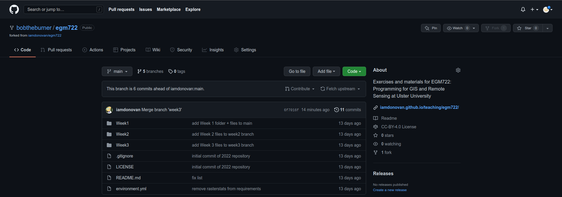
By now, you should have merged the week2 and week3 branches, so your main branch should look like this:

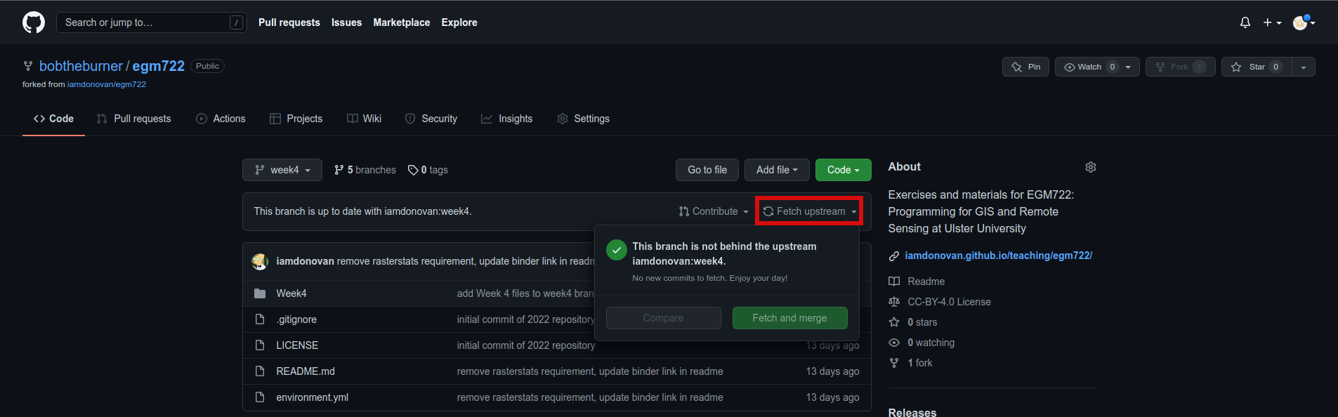
Like we saw last week, we can confirm that there aren’t any changes in to the upstream week4 branch by switching to the week4 branch:

Note

If you don’t see “This branch is up to date with iamdonovan:week4”, you can fetch the upstream changes by clicking the dropdown menu:

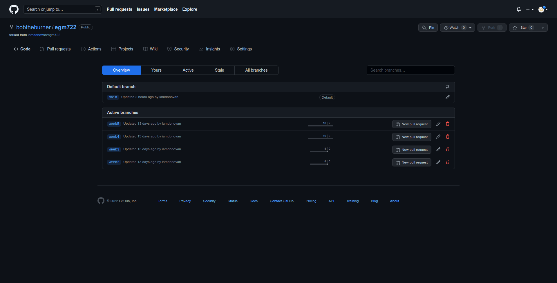
There are a number of different ways to actually open a Pull Request. From the branches page (https://github.com/<your_username>/egm722/branches), you can open a Pull Request for a specific branch by clicking the button next to that branch:

Otherwise, you can click on the Pull Requests tab:

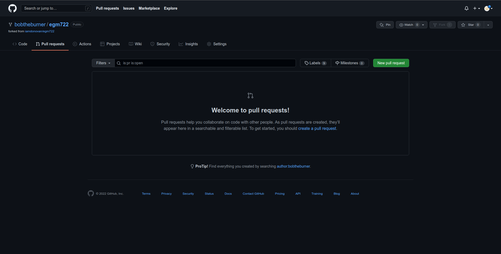
and click on the green New pull request button to start a new pull request:

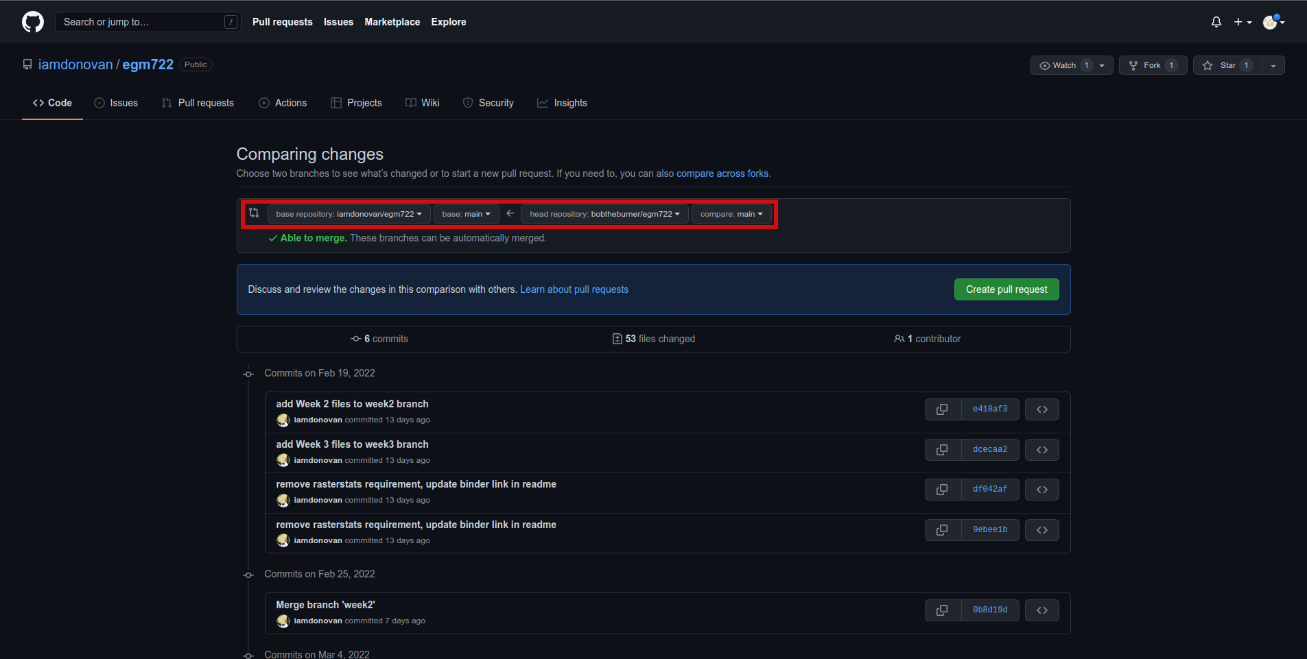
Note that the default behavior may be to try to merge from your fork into the upstream repository, so make sure that you’re attempting to merge the correct branches. You’ll need to change the branch that you’re merging into to <your_username>/egm722:main, and the branch that you’re merging from to <your_username>/egm722:week4. It should look like this:

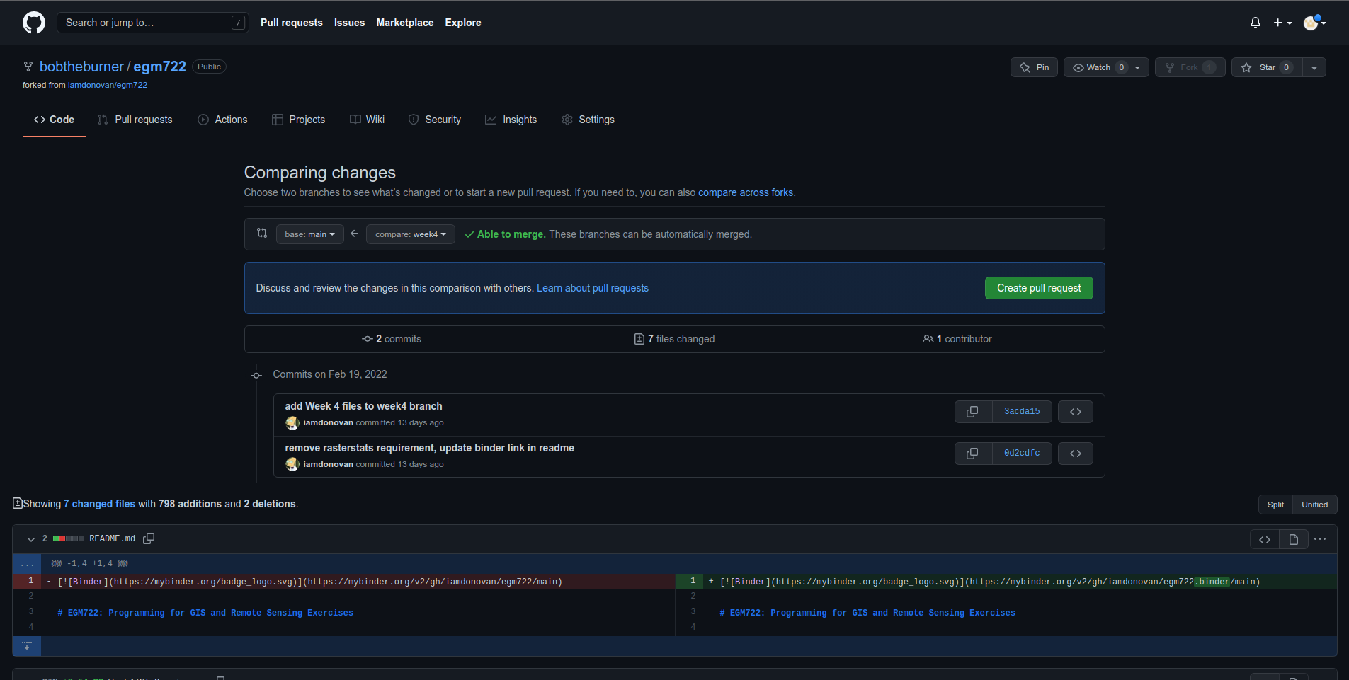
Once you’ve done this, scroll down to see the comparison showing which files have changed:

Here, deletions are shown on the left, while additions are shown on the right. For each file that has changed (either because it’s being added, or because it has been modified), you can see the summary of the changes in the upper left of each entry.

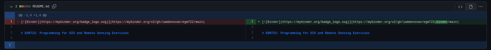
For this file, README.md, there have been 2 changes: 1 deletion and 1 addition (note that the current version may be slightly different).

Most of the changes that you see should be additions, since most of the files are only present on the week4 branch.

Once you’ve had a look at the comparison for the different files, you can click on the green Create pull request button, which will take you to the following page:

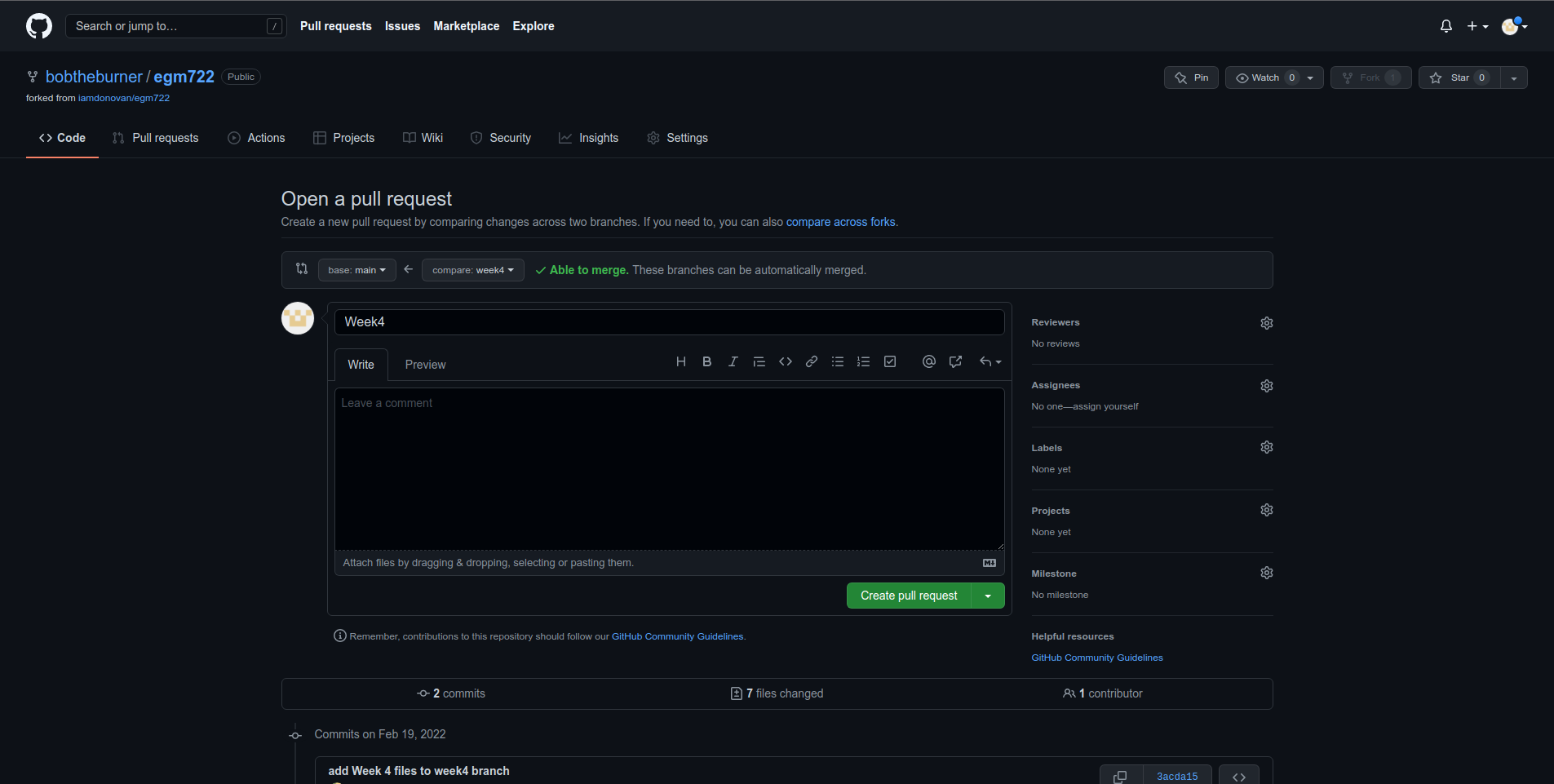
Depending on the project and repository settings, the pull request might need to be reviewed by others before it can be approved. The Message field above allows you to explain what the proposed changes are and why they should be approved.

Since you’re only making a change on your repository, you can leave this blank (though it’s good practice to explain what you’re doing in case you ever have to review what you’ve done – future you will thank you…).

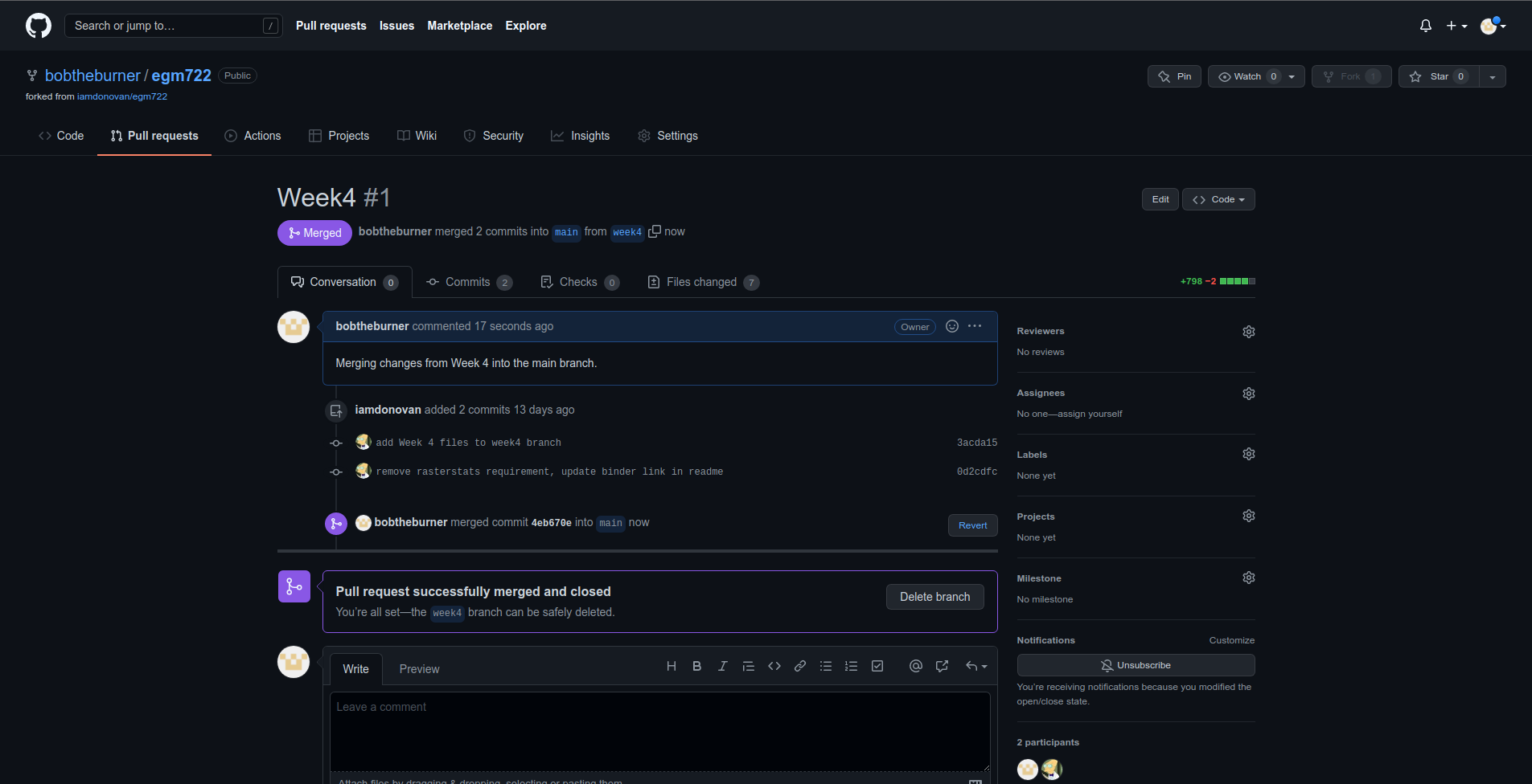
Once you’ve written the message, you can press the Create pull request button. As long as there aren’t conflicting changes (lines that have been changed in both branches), you should be able to merge the pull request by clicking the Merge pull request button:

You should then see the following screen, indicating that the two branches have been successfully merged:

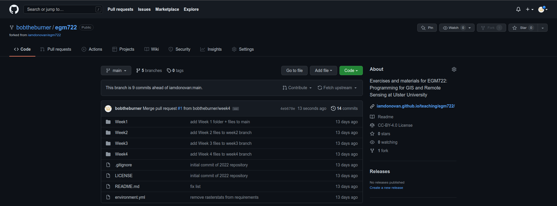
If you head back to the main repository page, you should see that the changes have been merged:

Now, on your computer, you can pull the changes to your machine using either GitHub Desktop or the command line:

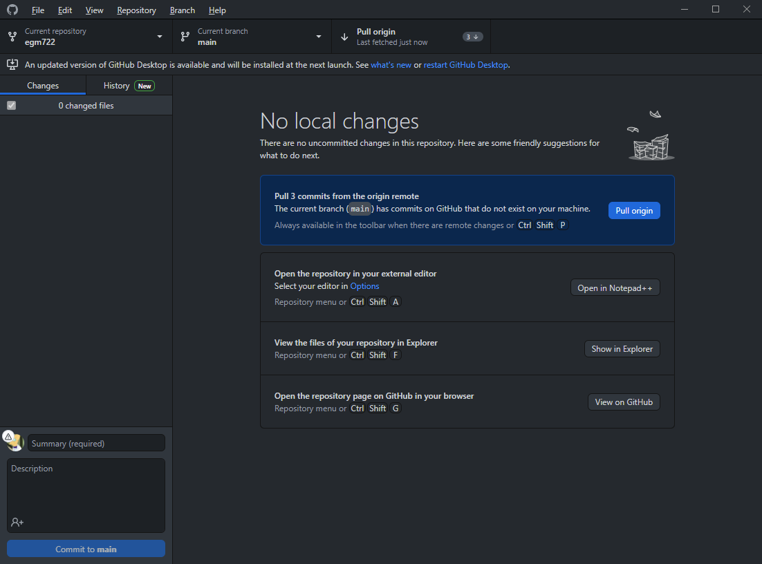
At this point, you can launch Jupyter Notebooks as you have in the previous weeks, and begin to work through the practical exercise.

Note

Below this point is the non-interactive text of the notebook. To actually run the notebook, you’ll need to follow the instructions above to open the notebook and run it on your own computer!

---

James Garner

overview

Up to now, you have gained some experience working with basic features of python, used cartopy and matplotlib to create a map, and explored using shapely and geopandas to work with vector data. In this week’s practical, we’ll be looking at working with raster data using rasterio and numpy.

objectives

• Learn about opening and viewing raster data using rasterio and cartopy

• Become familiar with opening files using a with statement

• Use * and ** to unpack arguments in a function

• Use rasterio to reproject raster data

data provided

In the data_files folder, you should have the following files: - NI_mosaic.tif

getting started

In this practical, we’ll be working with raster data. As a quick refresher, raster data are gridded datasets that contain anything from aerial and satellite images to elevation, temperature, or classisfied land cover. A raster is made up of pixels (or cells), where each pixel value represents the dataset’s value at a given location.

To get started, run the following cell to import rasterio and matplotlib.

%matplotlib inline

import numpy as np
import rasterio as rio
import cartopy.crs as ccrs
import matplotlib.pyplot as plt

In the box below, we load the dataset using rio.open() (documentation), then view some of the attributes of the dataset.

rio.open() creates a DatasetReader object (documentation) that we use to read the dataset and its attributes. When we do this, we don’t actually load the full raster into memory - we just open the file and read the metadata and other attributes. Later on, we’ll load the raster into memory; for now, we’ll look at the different attributes of the DatasetReader object.

For starters, the .name attribute is the filename for the dataset, and the .mode refers to how the dataset has been opened (r for read, w for write, r+ for read/write). We can also check how many layers, or bands, the datset has using .count, and check the size of the image using .width and .height. Finally, we can see the different types of data (e.g., integer, floating point, etc.) that each band has using .dtypes:

dataset = rio.open('data_files/NI_Mosaic.tif')

print('{} opened in {} mode'.format(dataset.name,dataset.mode))
print('image has {} band(s)'.format(dataset.count))
print('image size (width, height): {} x {}'.format(dataset.width, dataset.height))
print('band 1 dataype is {}'.format(dataset.dtypes[0])) # note that the band name (Band 1) differs from the list index [0]

We can also look at the georeferencing information for the dataset. The .bounds attribute gives locations for the left, bottom, right, and top sides of the image:

print(dataset.bounds)

Note that these values are in the coordinate reference system (CRS) of the dataset, which we can view using the .crs attribute - just like we have seen already with GeoDataFrame objects:

print(dataset.crs)

You should hopefully see that this dataset has a CRS of EPSG:32629, which corresponds to WGS84 UTM Zone 29N.

Finally, the .transform of a dataset is a 3x3 affine transformation matrix:

print(dataset.transform)

The maps pixel locations to real-world coordinates. The matrix has the following form:

| a b c |
| d e f |
| g h i |

where:

• a corresponds to the pixel width;

• b is the row rotation (normally 0);

• c is the x coordinate of the upper-left corner of the image;

• d is the column rotation (normally 0);

• e is the pixel height;

• f is the y coordinate of the upper-left corner of the image;

• g

• h

• i

loading the data

To load the data, we use the .read() method (documentation) of the DatasetReader object. This returns a numpy array (documentation):

img = dataset.read()

By default, .read() will load all of the bands associated with the dataset. To load specific bands, we can pass individual indices, or a list of indices, that we want to load (e.g., dataset.read(1) to load the first band or dataset.read([1, 2]) to load the first 2 bands).

Note that when we pass indices to the .read() method, we start indexing from 1, rather than 0. This is not the case for the array that is returned, however - here, the indices start from 0 (because python).

This can be confusing, so it’s important to pay attention to what kind of object you are working with when you start indexing.

print(img.shape) # returns a tuple with the number of image bands bands, image height, and image width.
print(img[7]) # will return an IndexError, because while there are 7 bands, the indices range from 0 to 6.

If we want to get a specific pixel value from the raster, we can index the array just like we would a list or tuple.

For example, to get the value of the center pixel in Band 1, we can do the following. For the arrays that we are using, the first index corresponds to the band (if there’s more than one band), the second index (first index if there’s only one band) corresponds to the row (y) location, and the third (second) index corresponds to the column (x) location:

print(img[0, dataset.height // 2, dataset.width // 2]) # note that // performs floor division, as indices have to be integers

Using the DatasetReader object, we can also find the pixel indices corresponding to spatial locations, and vice-versa, using both the .index() method (documentation) and the .transform attribute.

Note that the spatial locations should be in the same CRS as the image transform - if they are not, the image indices returned might not make sense:

centeri, centerj = dataset.height // 2, dataset.width // 2 # note that centeri corresponds to the row, and centerj the column
centerx, centery = dataset.transform * (centerj, centeri) # note the reversal here, from i,j to j,i
print(dataset.index(centerx, centery)) # show the indices that correspond to our x,y values
print((centeri, centerj) == dataset.index(centerx, centery)) # check that these are the same

If we don’t want to load the whole image at once, we can also choose a window using .read(). The format for this is a tuple of tuples corresponding to the top/bottom indices and left/right indices of the window. We can combine this with .index() to load a subset of the image based on spatial location (for example, using a vector dataset).

Here, we can select a 1 km window around the center pixel:

top, lft = dataset.index(centerx-500, centery+500)
bot, rgt = dataset.index(centerx+500, centery-500)

subset = dataset.read(window=((top, bot), (lft, rgt))) # format is (top, bottom), (left, right)

the with statement

Run the cell below to show the current status of our DatasetReader object:

dataset # show the current status of the dataset object

Here, we can see that the file is open, with a mode r indicating that we’re able to read the contents of the file on the disk.

Once we are done with the file (either reading, writing, appending, or whatever it happens to be), we have to remember to close the file using the .close() method:

dataset.close() # remember to close the dataset once we've read in what we need

Now, when we look at the current status of the DatasetReader object, we should see a change:

dataset # show the current status of the dataset object

Now, the file is closed, and if we try to read any additional attributes from it, we can’t:

dataset.read() # will return a RasterioIOError, because the dataset is closed

In python, we use the built-in open() function (documentation) to open files on the disk, in almost exactly the same way that rasterio.open() works. This allows us to work with the contents of the file - but, we always have to remember to close the file (using the .close() method) when we are done with it - otherwise, we may run into trouble later on.

f = open('my_file.txt', 'w')
...
f.close()

However, sometimes things happen. For example, an exception might be raised, or the interpreter might crash, and the file might stay open.

One way that we can handle opening/closing files without having to remember to explicitly close them is using a with statement:

with open('my_file.txt', 'w') as f:
    ...

This works exactly the same as what’s written above - within the with statement, we can use the variable f exactly as we would in the other example. As soon as the python interpreter reaches the end of the with block, it closes the file so that we don’t have to remember to do this.

In the cell below, we can re-open the dataset, extract the different attributes that we will need for the next few exercises, and then close the file:

with rio.open('data_files/NI_Mosaic.tif') as dataset:
    img = dataset.read()
    xmin, ymin, xmax, ymax = dataset.bounds

You should see that dataset is once again a closed DatasetReader object, even though we didn’t explicitly close it after opening it this time:

dataset # show the current status of the dataset object

displaying raster data using matplotlib and cartopy

Now that we’ve loaded our image, we can use cartopy and matplotlib to display it, just like we did for mapping vector data in Weeks 2 and 3.

To start, we’ll create a new cartopy CRS object (documentation), and use this to create a matplotlib Figure and Axes objects using matplotlib.pyplot.subplots() (documentation):

ni_utm = ccrs.UTM(29) # note that this matches with the CRS of our image
fig, ax = plt.subplots(1, 1, figsize=(10, 10), subplot_kw=dict(projection=ni_utm))

Now, we will use ax.imshow() (documentation) to display a single band from our image.

We’ll use the Landsat Near Infrared band - for our image, which is based on Landsat 5 TM images, this is Band 4 (which means that this corresponds to index 3 of our bands array):

ax.imshow(img[3], cmap='gray', vmin=200, vmax=5000) # display band 4 as a grayscale image, stretched between 200 and 5000
ax.set_extent([xmin, xmax, ymin, ymax], crs=ni_utm) # set the extent to the image boundary

fig # show the figure

As you can see from the link above, imshow() has a number of arguments that we can use to display our image. As we are using only a single band, we can set the minimum (vmin) and maximum (vmax) values of the image to stretch the display to, as well as what colormap to use (cmap). For more information about colormaps, you can check out this tutorial, as well as a recent paper on the (mis)use of color in science.

But, notice what happens when we use ax.set_extent() (documentation) to set the image extent - our image is nowhere to be seen!

By default, ax.imshow() uses the row/column indices of the image, rather than the geographic or projected coordinates of the raster. This means that we have to tell ax.imshow() both the tranform (CRS) to use, as well as the extent of the image, in order for it to display correctly.

Run the cell below - this time, you should see the image displayed in the correct location on the map after we set the Axes extents.

ax.imshow(img[3], cmap='gray', vmin=200, vmax=5000, transform=ni_utm, extent=[xmin, xmax, ymin, ymax])
ax.set_extent([xmin, xmax, ymin, ymax], crs=ni_utm) # set the extent to the image boundary

fig

This is not the only way that we can display images, however. We can also display them as RGB color composites. Try the following code, which should display the first three bands of the image:

ax.imshow(img[0:3], transform=ni_utm, extent=[xmin, xmax, ymin, ymax])

fig

So that didn’t work - we get a TypeError with the following message:

TypeError: Invalid shape (3, 1500, 1850) for image data

Remember that dataset.read() loaded the raster as a raster with three dimensions:

• dimension 1: the bands

• dimension 2: the rows

• dimension 3: the columns

But, ax.imshow() expects that the image indices are in the order (rows, columns, bands). From the documentation, we also see that:

X: array-like or PIL image
    The image data. Supported array shapes are:

    (M, N): an image with scalar data. The values are mapped to colors using normalization and a colormap.
        See parameters norm, cmap, vmin, vmax.
    (M, N, 3): an image with RGB values (0-1 float or 0-255 int).
    (M, N, 4): an image with RGBA values (0-1 float or 0-255 int), i.e. including transparency.
    The first two dimensions (M, N) define the rows and columns of the image.

    Out-of-range RGB(A) values are clipped.

So, to show an RGB image, we also need to scale our image to have values between 0-1 (or 0-255).

Now, we could try do this each and every time that we want to display an image, but this makes for unreadable code and also increases the likelihood that we will make a mistake writing our code.

In other words, this is a perfect place to write a function:

def img_display(image, ax, bands, transform, extent):
    '''
    This is where you should write a docstring.
    '''
    # first, we transpose the image to re-order the indices
    dispimg = image.transpose([1, 2, 0])

    # next, we have to scale the image.
    dispimg = dispimg / dispimg.max()

    # finally, we display the image
    handle = ax.imshow(dispimg[:, :, bands], transform=transform, extent=extent)

    return handle, ax

In this example, we first use the .transpose() (documentation) method on our image array to re-order the indices. The order of the indices in the argument here means that instead of the index order being (band, row, column), the order will now be (row, column, band), which is what ax.imshow() is expecting.

Next, we scale the image using .max() (documentation) so that the new values of dispimage range from 0 to 1.

Finally, we use ax.imshow() to display the image, using the transform and extent passed to the function, before returning the values of handle and ax.

Run the cell below to apply this function - you should see an RGB image of Landsat TM bands 3, 2, 1 (index 2, 1, 0), corresponding to “true color”:

h, ax = img_display(img, ax, [2, 1, 0], ni_utm, [xmin, xmax, ymin, ymax])
fig # just to save you from scrolling back up to see

So that worked, but the image is very dark - this is because of the way that we “normalized” the values to fall between 0 and 1, using the maximum of all of the bands:

maxvals = [img[ind].max() for ind in range(dataset.count)]
print(maxvals)

From the code below, we see that not all of the bands have the same range of values. Bands 1-3 have fairly low maximum values (2500-4100), while Band 5 has the highest values of all, over twice as high as in bands 1-3.

Rather than normalizing using the maximum value of all of the bands, we might want to instead normalize based on the maximum value of a given band. However, that might still result in dark or washed-out images, depending on whether we have a few very bright pixels.

Let’s instead try a percentile stretch, which should give a bit nicer results:

def percentile_stretch(image, pmin=0., pmax=100.):
    '''
    This is where you should write a docstring.
    '''
    # here, we make sure that pmin < pmax, and that they are between 0, 100
    if not 0 <= pmin < pmax <= 100:
        raise ValueError('0 <= pmin < pmax <= 100')
    # here, we make sure that the image is only 2-dimensional
    if not image.ndim == 2:
        raise ValueError('Image can only have two dimensions (row, column)')

    minval = np.percentile(image, pmin)
    maxval = np.percentile(image, pmax)

    stretched = (image - minval) / (maxval - minval) # stretch the image to 0, 1
    stretched[image < minval] = 0 # set anything less than minval to the new minimum, 0.
    stretched[image > maxval] = 1 # set anything greater than maxval to the new maximum, 1.

    return stretched

Here, we have a few new things happening. In the function header, we have two parameters, pmin and pmax, that we provide default values of 0 and 100, respectively:

def percentile_stretch(image, pmin=0, pmax=100):
    ...

We’ve seen this before, but it’s worth re-stating here that if we call the function like this:

stretched = percentile_stretch(img)

It will use the default values for pmin and pmax. Using default values like this provides us a way to make sure that necessary parameters are always set, without us always having to remember to set them when we call a function.

Next, note the conditional statement at the beginning of the function:

# here, we make sure that pmin < pmax, and that they are between 0, 100
if not 0 <= pmin < pmax <= 100:
    raise ValueError('0 <= pmin < pmax <= 100')

This single statement checks the following things:

• that pmin >= 0 (because it’s a percentage),

• that pmin < pmax (because min < max),

• that pmax <= 100 (again, because it’s a percentage).

If any of these things are not true, we raise (documentation) a ValueError, with a message indicating what caused the error.

Next, we have another conditional statement to check that our image only has two dimensions (i.e., that we are operating on a single band). To do this, we check that the number of dimensions (ndim) is equal to 2 - if it is not, we again raise a ValueError:

# here, we make sure that the image is only 2-dimensional
if not image.ndim == 2:
    raise ValueError('Image can only have two dimensions (row, column)')

After that, we use np.percentile() (documentation) to calculate the percentile value of the image for the values of pmin and pmax:

minval = np.percentile(image, pmin)
maxval = np.percentile(image, pmax)

Then, we stretch the image to values between 0 and 1:

stretched = (image - minval) / (maxval - minval) # stretch the image to 0, 1

and make sure to set any values below our minimum/maximum values to be equal to 0 or 1, respectively:

stretched[image < minval] = 0 # set anything less than minval to the new minimum, 0.
stretched[image > maxval] = 1 # set anything greater than maxval to the new maximum, 1.

Now, we should remember to update img_display() to use percentile_stretch(), so that the when we run img_display() again it applies our percentile stretch:

def img_display(image, ax, bands, transform, extent, pmin=0, pmax=100):
    '''
    This is where you should write a docstring.
    '''
    dispimg = image.copy().astype(np.float32) # make a copy of the original image,
    # but be sure to cast it as a floating-point image, rather than an integer

    for b in range(image.shape[0]): # loop over each band, stretching using percentile_stretch()
        dispimg[b] = percentile_stretch(image[b], pmin=pmin, pmax=pmax)

    # next, we transpose the image to re-order the indices
    dispimg = dispimg.transpose([1, 2, 0])

    # finally, we display the image
    handle = ax.imshow(dispimg[:, :, bands], transform=transform, extent=extent)

    return handle, ax

Now, run the new function, using a value of 0.1 for pmin and 99.9 for max (giving us a 99.8% stretch):

h, ax = img_display(img, ax, [2, 1, 0], ni_utm, [xmin, xmax, ymin, ymax], pmin=0.1, pmax=99.9)
fig # just to save you from scrolling back up to see

That looks much better - we can now see the image, it has good contrast, and the image is displayed in the correct location on the map.

functions with *args and **kwargs

At the moment, however, our function has a lot of extra parameters/arguments:

def img_display(image, ax, bands, transform, extent, pmin=0, pmax=100):
    ...

Rather than explicitly specifying the transform and extent each time, for example, we can change this to use the unpacking operators, * and **:

• * is used to unpack iterables - for example, a list or tuple

• ** is used to unpack keyword arguments - for example, using a dict

Let’s re-write our img_display() function to make use of these - first, by passing a list of percentile values to percentile_stretch() using *, and then by passing a dict of keyword arguments to pass to ax.imshow() using **:

def new_img_display(image, ax, bands, stretch_args=[0, 100], **imshow_args):
    '''
    This is where you should write a docstring.
    '''
    dispimg = image.copy().astype(np.float32) # make a copy of the original image,
    # but be sure to cast it as a floating-point image, rather than an integer

    for b in range(image.shape[0]): # loop over each band, stretching using percentile_stretch()
        dispimg[b] = percentile_stretch(image[b], *stretch_args) # pass the iterable stretch_args, but unpack them when calling percentile_stretch

    # next, we transpose the image to re-order the indices
    dispimg = dispimg.transpose([1, 2, 0])

    # finally, we display the image
    handle = ax.imshow(dispimg[:, :, bands], **imshow_args)

    return handle, ax

Now, create a dict called disp_kwargs with keys extent and transform, using the values we passed to ax.imshow() previously. We can also define stretch, a list of percentile values to pass to new_img_display():

disp_kwargs = {'extent': [xmin, xmax, ymin, ymax],
               'transform': ni_utm}

stretch = [0.1, 99.9] # a list of percentile values

h, ax = new_img_display(img, ax, [2, 1, 0], stretch_args=stretch, **disp_kwargs)
fig

You should see that this is the same image as before - the only thing that’s changed is how we call the function.

Feel free to try different stretch values, to see how it changes the image. If you’re interested in learning more about Landsat band combinations and image enhancement in general, you are welcome to watch the lecture videos provided by these links.

In the cell below, write some additional code to include gridlines for the map - if you don’t remember how, check back to the Week 2 Cartopy exercise to refresh your memory

# write your code here!

reprojecting rasters using rasterio

Fortunately, our image was provided in a geographic format that matches what we’ve been working with (WGS84 UTM Zone 29N). But, what if we need to have our image in a different format? In that case, we can use the rasterio.warp sub-module to reproject the image. The example below comes directly from an example provided in the rasterio documentation, and it makes use of two concepts that we’ve introduced in this practical: the with statement, *args, and **kwargs.

For more details about the different functions, such as rasterio.warp.calculate_default_transform() or rasterio.warp.reproject, check out the documentation.

The first part of this example:

with rio.open('data_files/NI_Mosaic.tif') as src:
    transform, width, height = rio.warp.calculate_default_transform(
            src.crs, dst_crs, src.width, src.height, *src.bounds)

opens the NI_Mosaic.tif file, and finds the new transform, width, and height attribute values for the reprojected (output) raster.

Next, we copy the meta attribute, a dict object, from the source dataset:

kwargs = src.meta.copy()

In order to match the output dataset, we use the .update() method (documentation) to change some of the attributes of the dict object before passing it to rio.open():

kwargs.update({
    'crs': dst_crs,
    'transform': transform,
    'width': width,
    'height': height
})

Finally, we open the new (reprojected) dataset, and reproject each band from the source dataset to the output dataset, using a nearest-neighbor resampling (Resampling.nearest):

with rio.open('data_files/NI_Mosaic_ITM.tif', 'w', **kwargs) as dst:
    for ind in range(1, src.count + 1): # ranging from 1 to the number of bands + 1
        rio.warp.reproject(
            source=rio.band(src, ind),
            destination=rio.band(dst, ind),
            src_transform=src.transform,
            src_crs=src.crs,
            dst_transform=transform,
            dst_crs=dst_crs,
            resampling=rio.warp.Resampling.nearest)

Note that this example only reprojects the raster from one CRS to another. If we wanted to, say, reproject the raster while also changing the pixel size or cropping to a particular data frame, we would need to calculate the new transform, width, and height values accordingly.

import rasterio.warp # note: we will be able to use rio.warp here, since we've previously imported rasterio as rio.
dst_crs = 'epsg:2157' # irish transverse mercator EPSG code

with rio.open('data_files/NI_Mosaic.tif') as src:
    transform, width, height = rio.warp.calculate_default_transform(
            src.crs, dst_crs, src.width, src.height, *src.bounds)
    kwargs = src.meta.copy() # this copies the meta dict object
    kwargs.update({
        'crs': dst_crs, # set the output crs
        'transform': transform, # set the output transform
        'width': width, # set the output width
        'height': height # set the output height
    }) # note: to change the values in a dictionary, we use the update() method

    with rio.open('data_files/NI_Mosaic_ITM.tif', 'w', **kwargs) as dst:
        for ind in range(1, src.count + 1): # ranging from 1 to the number of bands + 1
            rio.warp.reproject(
                source=rio.band(src, ind),
                destination=rio.band(dst, ind),
                src_transform=src.transform,
                src_crs=src.crs,
                dst_transform=transform,
                dst_crs=dst_crs,
                resampling=rio.warp.Resampling.nearest)

next steps

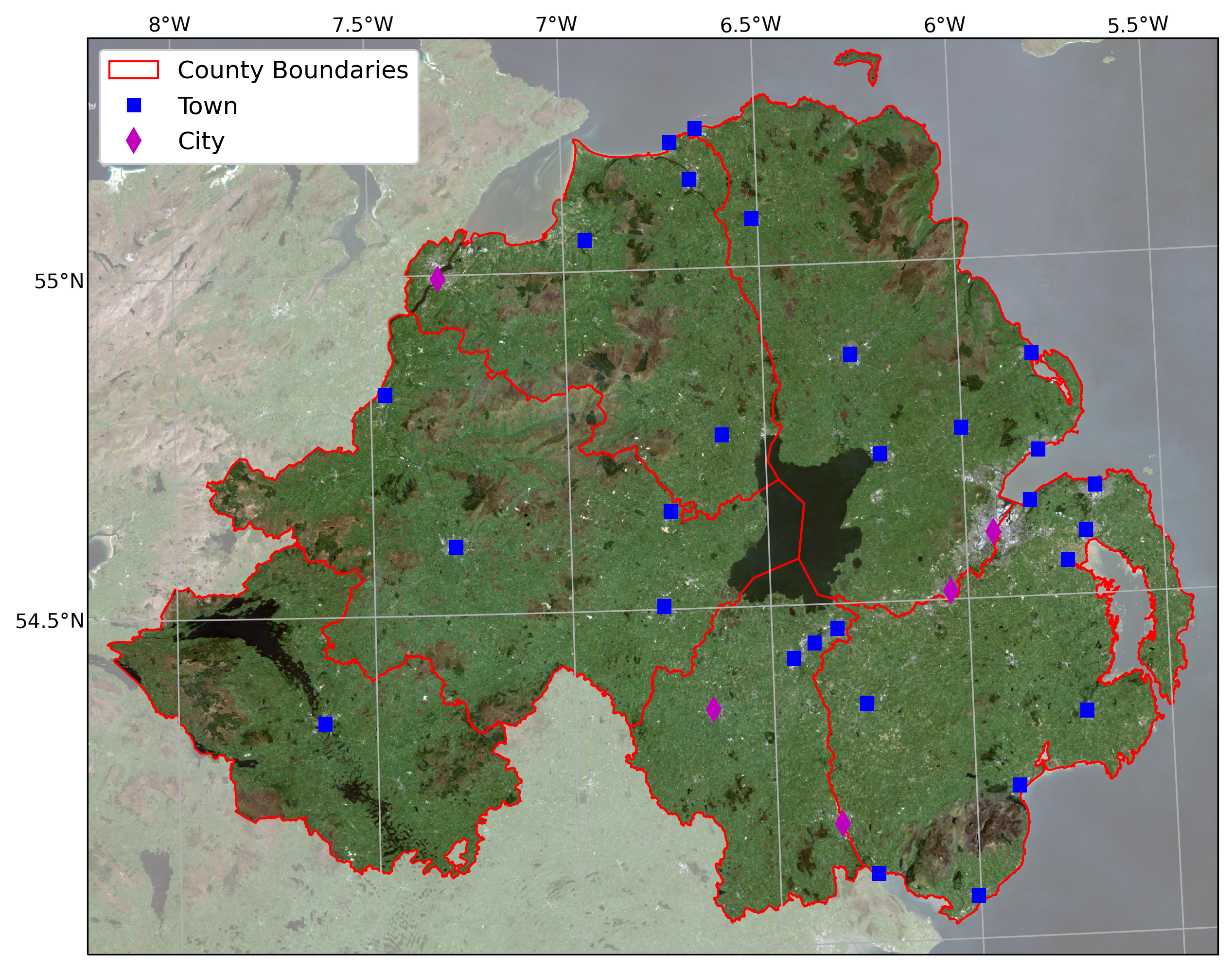
For some additional practice with the concepts covered in this practical, use the assignment_script.py file in the Week4 folder to work on a script that combines the concepts we’ve used this week, as well as some of the material from previous weeks, to produce a map that overlays the county borders and town/city locations on the satellite image provided.

For an additional challenge, try this: In the image below, notice how the area outside of the county borders has been covered by a semi-transparent overlay. Can you work out a way to do this? Check over the import statements in assignment_script.py carefully - there’s at least one import that we haven’t discussed yet, but it should help point you in the right direction.

I’ll provide my example next week, but try to think about the different steps involved and how you might solve this, using some of the examples provided in previous weeks. Good luck!