basic statistical analysis using python#
Note
This is a non-interactive version of the exercise. If you want to run through the steps yourself and see the outputs, you’ll need to do one of the following:
follow the setup steps and work through the notebook on your own computer
open the workshop materials on binder and work through them online
open a python console, copy the lines of code here, and paste them into the console to run them
In this exercise, we’ll take a look at some basic statistical analysis
with python - starting with using python and pandas to calculate
descriptive statistics for our datasets, before moving on to look at a
few common examples of hypothesis tests using pingouin.
data#
The data used in this exercise are the historic meteorological observations from the Armagh Observatory (1853-present), the Oxford Observatory (1853-present), the Southampton Observatory (1855-2000), and Stornoway Airport (1873-present), downloaded from the UK Met Office that we used in previous exercises. I have copied the combined_stations.csv data into this folder - this is the same file that you created in the process of working through the “pandas” exercise.
loading libraries#
First, we’ll import the various packages that we will be using here:
pandas, for reading the data from a file;
seaborn, for plotting the data;
pingouin, for the statistical tests that we’ll use;
pathlib, for working with filesystem paths.
import pandas as pd
import seaborn as sns
import pingouin as pg
from pathlib import Path
Next, we’ll use pd.read_csv() to load the combined station data.
We’ll also use the parse_dates argument to tell pandas to read
the date column as a date:
station_data = pd.read_csv(Path('data', 'combined_stations.csv'), parse_dates=['date'])
descriptive statistics#
Before diving into statistical tests, we’ll spend a little bit of time
expanding on calculating descriptive statistics using pandas. We
have seen a little bit of this already, using .groupby() and
.mean() to calculate the mean value of rain for each station.
describing variables using .describe()#
First, we’ll have a look at .describe()
(documentation),
which provides a summary of each of the (numeric) columns in the table:
station_data.describe()
In the output above, we can see the count (count) minimum (min), 1st quartile (25%), median (50%), mean (mean), 3rd quartile (75%), maximum (max), and standard deviation (std) values of each numeric variable.
With this, we can quickly see where we might have errors in our data -
for example, if we have non-physical or nonsense values in our
variables. When first getting started with a dataset, it can be a good
idea to check over the dataset using .describe().
using .describe() to summarize groups#
What if we wanted to get a summary based on some grouping - for example,
for each station? We could use filter() to create an object for each
value of station, then call summary() on each of these objects
in turn.
Not surprisingly, however, there is an easier way, using split()
(documentation) and map()
(documentation).
First, split() divides the table into separate tables based on some
grouping:
station_data.groupby('station').describe()
On its own, this output isn’t all that readable - the summary statistics
are put into individual columns, which means that the table is very
wide. Let’s see how we can re-arrange this so that we have a dict()
of DataFrames, one for each station. First, we’ll assign the output
of .describe() to a variable, group_summary:
group_summary = station_data.groupby('station').describe()
Next, we’ll iterate over the stations to work with each row of the table in turn. First, though, let’s look at how the column names are organized:
group_summary.columns # show the column names
This is an example of a MultiIndex
(documentation)
- a multi-level index object, similar to what we have seen previously
for rows. Before beginning the for loop below, we use
columns.unique()
(documentation)
to get the unique first-level names from the columns (i.e., the variable
names from the original DataFrame).
Inside of the for loop, we first select the row corresponding to
each station using .loc. Have a look at this line:
reshaped = pd.concat([this_summary[ind] for ind in columns], axis=1)
This uses something called list comprehension to quickly create a list of objects. It is effectively the same as writing something like:
out_list = []
for ind in columns:
    out_list.append(this_summary[ind])

reshaped = pd.concat(out_list, axis=1)
Using list comprehension helps make the code more concise and readable - it’s a very handy tool for creating lists with iteration. In addition to list comprehension, python also has dict comprehension - we won’t use this here, but it works in a very similar way to list comprehension.
Once we have reshaped the row (the Series) into a DataFrame, we
assign the column names, before using .append() to add the reshaped
table to a list:
stations = group_summary.index.unique() # get the unique values of station from the table
columns = group_summary.columns.unique(level=0) # get the unique names of the columns from the first level (level 0)

combined_stats = [] # initialize an empty list

for station in stations:
    this_summary = group_summary.loc[station] # get the row corresponding to this station

    reshaped = pd.concat([this_summary[ind] for ind in columns], axis=1) # use list comprehension to reshape the table
    reshaped.columns = columns # set the column names
    combined_stats.append(reshaped) # add the reshaped table to the list
Finally, we’ll use the built-in function zip() to get pairs of
station names (from station) and DataFrames (from
combined_stats), then pass this to dict() to create a dictionary
of station name/DataFrame key/value pairs:
summary_dict = dict(zip(stations, combined_stats)) # create a dict of station name, dataframe pairs
To check that this worked, let’s look at the summary data for Oxford:
summary_dict['oxford'] # show the summary data for oxford
using built-in functions for descriptive statistics#
This is helpful, but sometimes we want to calculate other descriptive
statistics, or use the values of descriptive statistics in our code.
pandas has a number of built-in functions for this - we have already
seen .mean()
(documentation),
for calculating the arithmetic mean of each column of a DataFrame:
station_data.mean(numeric_only=True) # calculate the mean for each numeric column
Series objects (columns/rows) also have .mean()
(documentation):
station_data['rain'].mean() # calculate the mean of the rain column
We can calculate the median of the columns of a DataFrame (or a
Series) using .median()
(documentation):
station_data.median(numeric_only=True) # calculate the median of each numeric column
To calculate the variance of the columns of a DataFrame (or a
Series), use .var()
(documentation):
station_data.var(numeric_only=True)
and for the standard deviation, .std()
(documentation):
station_data.std(numeric_only=True)
pandas doesn’t have a built-in function for the inter-quartile range
(IQR), but we can easily calculate it ourselves using .quantile()
(documentation)
to calculte the 3rd quantile and the 1st quantile and subtracting the
outputs:
station_data.quantile(0.75, numeric_only=True) - station_data.quantile(0.25, numeric_only=True)
Finally, we can also calculate the sum of each column of a DataFrame
(or a Series) using .sum()
(documentation):
station_data.sum(numeric_only=True)
These are far from the only methods available, but they are some of the
most common. For a full list, check the pandas
documentation
under Methods.
with .groupby()#
As we have seen, the output of .groupby() is a special type of
DataFrame, and it inherits almost all of the methods for calculating
summary statistics:
station_data.groupby('station').mean(numeric_only=True)
statistical tests#
In addition to descriptive statistics, we can use python for
inferential statistics - for example, for hypothesis testing. In the
remainder of the exercise, we’ll look at a few examples of some common
statistical tests and how to perform these in python, using
statsmodels. Please note that these examples are far from exhaustive
- if you’re looking for a specific hypothesis test, there’s a good
chance someone has programmed it into python, either as part of the
statsmodels package
(documentation), or
as part of scipy.stats
(documentation),
or as part of an additional package that you can install. You should be
able to find what you need with a quick internet search.
independent samples student’s t-test#
For a start, let’s test the hypothesis that Stornoway Airport gets more rain than Armagh. If we first have a look at a box plot:
selected = station_data.loc[station_data['station'].isin(['stornoway', 'armagh'])] # select stornoway airport and armagh data

sns.boxplot(data=selected, x='station', y='rain')
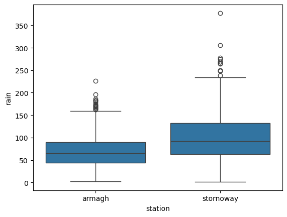
It does look like Stornoway Airport does get more rain, on average, than Armagh.
To run Student’s t-test using pingouin, we use pg.ttest()
(documentation):
armagh_rain = selected.loc[selected['station'] == 'armagh', 'rain'].dropna().sample(n=30) # take a sample of 30 rain observations from armagh
stornoway_rain = selected.loc[selected['station'] == 'stornoway', 'rain'].dropna().sample(n=30) # take a sample of 30 rain observations from stornoway

# test whether stornoway_rain.mean() > armagh_rain.mean() at the 99% confidence level
rain_comp = pg.ttest(stornoway_rain, armagh_rain, alternative='greater', confidence=0.99)

rain_comp # show the results dataframe
The output of pg.ttest() is a DataFrame that gives us the
following:
T: the value of the t-statistic;dof: the degrees of freedom;alternative: the hypothesis that was used;p-val: the p-value of the t-statistic;CI{confidence}%: the confidence interval for the chosen significance level;cohen-d: Cohen’s d effect size;BF10: the Bayes Factor of the alternative hypothesis;power: the achieved power of the test
Now, let’s look at an example of a one-sample t-test, to see if we can determine whether the mean of a small sample of summer temperatures provides a good estimate of the mean of all summer temperatures measured at Oxford.
First, we’ll select all of the summer values of tmax recorded at
Oxford, then calculate the mean value of these temperatures:
oxford_summer_tmax = station_data.query('station == "oxford" & season == "summer"')['tmax']

print(f"Oxford Mean Summer Tmax: {oxford_summer_tmax.mean():.1f}")
So the mean summer temperature measured in Oxford between 1853-2022 is
21.1°C - now, let’s take a random sample of 30 temperatures using
.sample():
sample_tmax = oxford_summer_tmax.sample(n=30) # select a random sample of 30 values
Once again, we use pg.ttest() to conduct the test. Because
oxford_summer_tmax is a single value, the function knows that this
is a one-sample test:
# test whether sample_tmax.mean() is not equal to oxford_summer_tmax at the 95% confidence level
tmax_comp = pg.ttest(sample_tmax, oxford_summer_tmax, alternative='two-sided', confidence=0.95)

tmax_comp # show the results dataframe
Based on this, we can’t conclude that our sample mean is significantly
different from the mean of all of the summer values of tmax recorded
at Oxford.
non-parametric tests#
We can also conduct non-parametric hypothesis tests using pingouin.
The example we will look at is the one- or two-sample Wilcoxon tests,
using pg.wilcoxon()
(documentation).
Let’s start by looking at the Wilcoxon Rank Sum test, which is analogous
to the independent sample t-test. For this, we’ll use the same data
that we did before, again testing whether Stornoway Airport gets more
rainfall, on average, than Armagh:
# test whether mean(stornoway.rain) > mean(armagh.rain)
pg.wilcoxon(stornoway_rain, armagh_rain, alternative='greater')
The output table has the following columns:
W-val: the W-statistic of the test;alternative: the alternative hypothesis uesd;p-val: the p-value of the W-statistic;RBC: the matched pairs rank-biserial correlation (i.e., the effect size);CLES: the common language effect size.
From this, we can again conclude that Stornoway Airport does get more rainfall, on average, than Armagh.
analysis of variance#
Finally, we’ll see how we can set up and interpret an analysis of
variance test. In this example, we’ll only look at data from Armagh,
Oxford, and Stornoway Airport, because the Southampton time series ends
in 1999. We’ll first calculate the annually-averaged values of the
meteorological variables, using .groupby() and .mean():
annual_average = station_data.loc[station_data['station'].isin(['armagh', 'oxford', 'stornoway'])] \
    .groupby('year') \
    .mean(numeric_only=True)
Then, we’ll add a new variable, period, to divide the observations
into three different 50-year periods: 1871-1920, 1921-1970, and
1971-2020. To do this, we’ll use pd.cut() (documentation). To
do this, we first have to define the labels (periods) and category
boundaries (bins). Then, we use .dropna() to remove any rows
where period has a NaN value (i.e., is outside of the range
1871-2020):
periods = ['1871-1920', '1921-1970', '1971-2020'] # make a list of period names
bins = [1870, 1920, 1970, 2020] # make a list of period boundaries - must be 1 longer than the names

annual_average['period'] = pd.cut(annual_average.index, bins, labels=periods) # assign a value to period, using the boundaries and labels above

annual_average.dropna(subset=['period'], inplace=True) # drop any rows where period is NaN

annual_average # show the dataframe
Before running the test, let’s make a box plot that shows the
distribution of tmax values among the three periods:
sns.boxplot(data=annual_average, x='period', y='tmax') # make a box plot of tmax, grouped by period
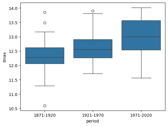
From this, it certainly appears as though there is a difference in the
mean value of tmax between the three periods. To formally test this,
we’ll use aov()
(documentation).
To run the one-way ANOVA test, we use pg.anova()
(documentation).
Using this, we can pass our annual_average DataFrame using the
data argument, and specify tmax as the dependent variable
(dv), and period as the grouping variable (between). We’ll
also look at the detailed test output (detailed=True):
aov = pg.anova(dv='tmax', between='period', data=annual_average, detailed=True) # run one-way anova for differences of tmax between periods

aov.round(3) # round the output to 3 decimal places
The table output has the following columns across two rows:
Source: the factor names;SS: the sums of squares;DF: the degrees of freedom;MS: the mean squares;F: the value of the F-statistic;p-unc: the uncorrected p-values;np2: the partial eta-square effect sizes
From the table, we can see that there are significant differences between the groups at the 99.9% significance level.
This doesn’t tell us which pairs of groups are different - for this, we
would need to run an additional test. As one example, we can use
pg.pairwise_tukey()
(documentation)
to compute “Tukey’s Honest Significant Difference” between each pair of
groups:
tmax_mc = pg.pairwise_tukey(dv='tmax', between='period', data=annual_average) # run the pairwise tukey HSD post-hoc test

tmax_mc.round(3) # round the output to 3 decimal places
From this, we can see the estimated difference in the means for each
pair of groups (shown in A and B); the estimated mean of each
group; the estimated difference between the mean of each group
(diff); the standard error of the estimate (se); the
t-statistic of the estimated difference (T); the corrected
p-value of the t-statistic (p-tukey), and the effect size (by
default, Hedges).
Using this, we can clude that, at the 99% significance level, there is a
significant difference in tmax between the periods 1971-2020 and
1871-2020, and between the periods 1971-2020 and 1921-1970.
exercise and next steps#
That’s all for this exercise. To help practice your skills, try at least one of the following:
Set up and run an AOV test to compare annual total rainfall at all four stations, using data from all avaialable years. Are there significant differences between the stations? Use
pg.pairwise_tukey()orpg.pairwise_tests()(documentation) to investigate further.Using only observations from Armagh, set up and run a test to see if there are significant differences in rainfall based on the season.
Using only observations from Oxford, is there a significant difference between the values of
tmaxin the spring and the autumn at the 99.9% confidence level?Using only observations from Stornoway Airport, is the value of
tminsignificantly lower in the winter, compared to the autumn?